This unit requires students to apply simple exponential functions in everyday situations.
- Create a table of values based on an exponential relationship.
- Graph an exponential relationship on a number plane.
- Create an equation for a simple exponential function.
- Recognise the effect of the size of base on the growth or decay curve for an exponential function.
- Apply exponential functions to everyday situations.
In this unit students build on their knowledge of exponents to investigate situations where exponential change occurs. Typically, those situations involve a fixed ratio between consecutive members of a geometric sequence. The ratio is the base of the exponential function, and that ratio is applied 'n' times to find the nth member of the sequence.
For example, suppose $100 is invested at an interest rate of 5% per annum. At the end of year 1 an additional $5 in interest will be earned. The total amount in the bank is $105. The ratio between 105 and 100 is 1.05, which is the base of the exponential relationship between number of years and amount in the bank. By the end of the fifth year the base, 1.05, will have been applied five times so the amount will be 100 x 1.05 x 1.05 x 1.05 x 1.05 x 1.05. This can be simplified to 100 x (1.05)5. In general, the amount of money after year n is y = 100(1.05)n.
In general, exponential functions are of the form y = a(b)x though transformations can also be applied (translations and reflections). A represents the quantity of term zero and b is the base. Most situations in this unit are about discrete relationships in which integral values for one variable relate exponentially to integral values of the other variable. Exponential functions are generally continuous meaning the variables are free to take up any value in the domain of the function, e.g. temperature of a forest fire as time increases.
The learning opportunities in this unit can be differentiated by providing or removing support to students and by varying the task requirements. Ways to support students include:
- modelling the construction of graphs, tables, and the entry of data into spreadsheets
- providing pre-prepared tables and graphing templates for students to fill out
- grouping students flexibly to encourage peer learning, scaffolding, extension, and the sharing and questioning of ideas
- applying gradual release of responsibility to scaffold students towards working independently
- providing frequent opportunities for students to share their thinking and strategies, ask questions, collaborate, and clarify in a range of whole-class, small-group, peer-peer, and teacher-student settings.
The context for this unit can be adapted to suit the interests and experiences of your students. Select contexts that involve doubling of quantities, the population of animals, percentage growth, etc. that are relevant to your students. Perhaps you could generate a list of contexts with your class.
Te reo Māori kupu such as ōrau (percent), taupūtanga (exponential), and whārite (equation) could be introduced in this unit and used throughout other mathematical learning.
Getting Started
- Use PowerPoint One to introduce the concept of exponential growth. Slide One shows a growth pattern in wealth depicted graphically.
What is the slide representing?
- Students might focus on the pattern by which the number of coins is increasing (doubling with each step to the right).
Suppose the number of coins relates to Natasha’s years of investing. Create a table of years and her worth in coins.
You might start the table like this:
| Year | Worth |
| 0 | 1 |
| 1 | 2 |
| 3 | ? |
| … | … |
- Let students create their tables and check the values against the picture on Slide One.
What could we say about how Natasha’s worth is growing?
What percentage growth is she achieving each year? (100%)
How steeply is her worth growing? (The difference in stacks between years gets greater and greater)
How long will it take for Natasha to become a millionaire?
- Let students work on the final question in pairs using a calculator. By repeatedly doubling, students will arrive at an amount greater than $1,000,000. However, it is important for them to track the year numbers as they work. The relationship between values of two variables is at the heart of function as a concept. In the 20th year Natasha’s wealth hits $1,048,576.
Each one-dollar coin is 2.74 mm thick. I wonder how high is the stack?
1 048 576 x 2.74 = 2 873 098.24mm. That’s 2 873 metres (rounding) which is 2.87 kilometres!
Slide two shows how a graph of the relationship between year number and Natasha’s worth is created. The video uses Desmos as the platform but it is very important for the students to create the graph manually using graph paper. Look for your students to:
- Establish sensible scales on the axes, especially the y-axis that represents Natasha’s worth
- Label the axes appropriately, including referencing units
- Co-ordinate the values of both variables simultaneously in locating ordered pairs.
Slides three and four allow you to discuss different types of functions, that are many to one relationships, between the values of variables. The functions shown look similar in equation form, particularly y=x2 and y= 2x.
- Ask students to provide co-ordinates of points that lie on the functions. Success at that task indicates that students understand the transformations on discrete (individual) x-values that yield discrete y-values.
In the next part of the lesson we use an analogy from Professor David Suzuki, a world leader in sustainable ecology. You will easily find a video of a talk by David online. The idea is for students to understand the implication of exponential growth of the world population for a sustainable future.
- Work through 5-12 slides of PowerPoint One and discuss the analogy. Slide 12 has four questions for the students to answer. They will need copies of Copymaster One to answer question three. Look for your students to:
- Describe the similarity between bacterial growth and growth in the human population in terms of exponential change.
- Recognise that the resources of the Earth and the petrie dish are similarly finite.
- Describe how bacteria at minute 55 might believe there is no problem since nearly 97% of the food is spare and things have been fine for a long time (in bacteria minutes that is).
- Notice that the doubling time for the human population has varied since records began and that it can be changed. Estimates of that time changed from 37 years in 1998 to 95 years in 2008. Why?
- Take an informed stance on how the situation may be changed, e.g. reducing the number of children per family, reduce consumption, etc.
The final slide shows the trend over time (60 minutes) in the percentage of the food in the dish that the bacteria consume. Students should note the implications of exponential growth, the rapid change in percentage occurs over a short duration of minutes. You might look up graphs of human population growth to show a similar pattern over time.
Session 2
In this session students explore exponential functions where the base is one half. In that case the number of units of the dependent variable is multiplied by one half for each increase of one unit in the independent variable. The result is a repeated halving process. Exponential decay is used in real life to calculate the amount of a drug in a person’s bloodstream and to date the age of historical artefacts.
- Use PowerPoint Two to introduce the idea of half-life for drugs. In the simplified example the anaesthetic has a half-life of one hour. After reading through the first three slides watch the animation.
What is happening to the amount of the drug in the bloodstream every hour? (It is halving)
Work with a partner to predict the amount of drug present in the bloodstream after four, five, and six hours.
- Use the students’ answers to generate a table of values, like this:
| Time (hours) | 0 | 1 | 2 | 3 | 4 | 5 |
| Amount of drug (mg) | 100 | 50 | 25 | 12.5 | 6.25 | 3.125 |
Imagine we graphed these pairs of numbers as co-ordinates. What do you think the shape of the graph would be?
- Invite students to suggest possible shapes then provide graph paper and ask them to graph the six ordered pairs. Suggest the importance of labelling the axes and giving the graph a title. You might show Slide Four of PowerPoint Two to show how a graph can be created. It is important that students create the ordered pairs and graph them as individual points rather than simply creating a continuous graph with digital technology.
What do you think will happen to the points as you graph later times?
Students might believe that at some time the curve will cross the x-axis. Let them graph more points to establish that the curve converges to the x-axis but does not cross it. Introduce the idea of an asymptote which is a line in this case. The distance between the curve and line approaches zero as the values of the independent variable change. In this context, the amount of drug in the bloodstream approaches zero as the number of hours since injection increases.
- Using digital graphing tools (including graphics calculators) pose this challenge:
The curve can be represented by this equation: y=100(bx). Your job is to find out what b equals.
What do x and y represent in the equation? (x represents time in hours, y represents amount of the drug in milligrams)
Why is 100 in the equation? (The function begins at time zero when 100mg of the drug are injected)
- Let students investigate the effect of changes to b. They should discover that b values greater than one result in the type of growth curve seen in lesson one. A b value of one creates a straight line, y=1. Values of b less than one result in the exponential decay curve. In this case b = 0.5 or 1/2. The equation is y=100(1x/2) though the brackets are redundant due to order of operations. Slide Five presents three different curves.
Which equation matches each curve? How do you know?
Is anything the same about all three curves?
Since the scales are different it may be difficult for students to spot that the point (0, 1) is common to all three curves. You may need to work on lessons from the Level 5 unit, Exponent Power, to help students see why b0=1, for all values of b.
- Provide your students with Copymaster Two. This contains problems to solve with exponential functions where 0<b<1. There are two scenarios, decay of caffeine levels and cooling of water. The latter involves a slightly more complex function that uses the starting temperature and environmental temperature, but is simplified for students at Level Five (see Newton’s rule for cooling). Important points in Copymaster Two are:
- Curves of exponential decay functions have negative slopes that approach a gradient of zero, the functions are not linear.
- Ordered pairs can be estimated within the given data points. That process is called interpolation.
- Ordered pairs for data points beyond the given ordered pairs can be estimated by extending the curve of the graph in a consistent way. That process is called extrapolation.
- Caffeine has a half life of about six hours, so a quarter life of 12 hours, etc. The implication is that it stays in your system for a long time after consumption.
- Cooling of a container of water varies due to many factors such as surface area to volume, environment (room) temperature, insulation, etc. However, the function is exponential. The final challenge is possible by curve fitting with a graphing package. The equation y=480(0.89089x) is a good fit to the data. The base can be found using algebra that is beyond Level Five.
Session Three
So far students have explored exponential functions with bases of two, and one half, though that was extended in Lesson Two. In this lesson students experiment the effect of changing the base. They do so through two contexts; Lock combinations and management trees.
Part One: Combination Locks
- Use PowerPoint Three Slides One to Three to introduce the security scheme used on Melbourne’s open access bicycle scheme. Discuss why the security was needed. The designer needed to balance the security of the bicycles with the ease of use of the codes. If it was too easy to enter the code by chance thieves might steal the bicycles. If the code was too hard to use people would make errors keying in the number and the code would need to be reset.
After slide two ask:
How can you work out the chance of entering the correct code by luck? (Need to find all the possible permutations)
What are some ways to find all the possible codes? (Create a systematic list, a tree diagram, etc.)
- Slide Three uses a tree diagram to find all the possible two-place codes with 1, 2, and 3 as the digits. Ask students to draw the tree diagram to three places.
How many different three place codes are possible? (27)
Why are there 27 possibilities? (3 x 3 x 3)
Is there a way to anticipate how many 5-place codes are possible for the Melbourne bicycles? (3 x 3 x 3 x 3 x 3 = 243)
The chances of getting the code by luck are 1/243, not high. How many codes would be possible if the managers increased the number of places to six, seven, or eight?
Why might they do that? Why might they not do that?
- Make a table to show the number of codes that are possible as the number of places increases.
| Number of places | 1 | 2 | 3 | 4 | 5 | 6 | 7 |
| Number of possible codes | 3 | 9 | 27 | 81 | 243 | 729 | 2187 |
- Ask your students to graph the relationship.
Do they notice that the vertical scale needs to go from zero to 2200?
- Slide Four shows a graph of the relationship. Ask:
What equation would create a path that goes through these points? (y=3x where x represents the number of places, and y represents the number of codes)
- Use Slide Five to investigate what happens when the number of digits increases.
Imagine that the digits 1, 2, 3 and 4 are used, instead of 1, 2 and 3. What effect would that have? Create a table about the number of possible codes.
| Number of places | 1 | 2 | 3 | 4 | 5 | 6 | 7 |
| Number of possible codes | 4 | 16 | 64 | 256 | 1024 | 4056 | 16384 |
Imagine we graphed this relationship on the same graph as you used previously. What would happen? (Do the students realise that the vertical scale will not be nearly high enough?)
How much higher does the vertical scale need to be? (about eight times higher)
You might investigate the effect of changing the number of digits on the growth curve for the number of possible codes, graph the curves using digital technology, and write equations or curves that pass through the points.
- Use the problem on Slide Six as a collaborative task to see that students appreciate the effect of a change in base.
Part Two: Management Structures
- Use PowerPoint Three. Slides Six to Eight show how management structures are integral to businesses.
What is the downside of having few employees to every manager? (cost)
What is the downside of too many employees to every manager? (Supervision and communication are difficult and workload for the manager gets too high)
- At the end of Slide Nine ask:
Draw the diagram and add another layer. How many employees will be in the fourth layer? (27) How did you get that?
- Set up a table of values, like this:
| Layers of management | 0 | 1 | 2 | 3 | 4 | 5 |
| New employees | 1 | 3 | 9 | 27 | ? | ? |
How many new employees will be added in layers four, five and six?
How is situation similar and different to the number of the bacteria story?
Slide Ten shows a graph of the function and highlights the point (0,1), i.e. No layers but one manager. The curve shows the pattern of a path through the points. Note that the context is discrete, i.e. involves whole numbers of people, not continuous.
- Ask:
What do you think would happen to the curve if the ratio of managers to employees was 1:4?
Why would that happen?
Slide Eleven shows the curves for ratios of 1:3 and 1:4 on the same graph. Students should note that the difference between the number of new employees grows dramatically as the number of layers increases.
- Set up the scenario on Slides Twelve to Fourteen. Let the students explore the problem, preferably with the support of spreadsheets and calculators. There are various degrees of sophistication that might be used. Look for:
- Do they use a repeated multiplication formula to generate each sequence of powers?
- Do they recognise the number of layers needed before 10 000 employees is reached?
- Do they identify how many managers there will be?
More sophistication occurs when students recognise that the power immediately below 10 000 is significant. The sum of numbers of people before that power will all be managers. For example, look at the powers of five:
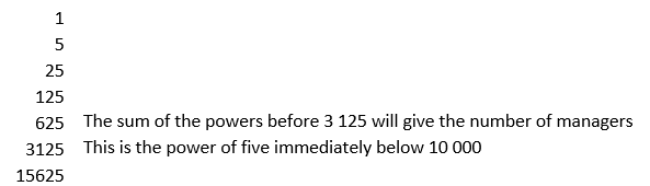
However, there will need to be another 6 875 employees to reach 10 000. They will need managers at a ratio of 1:5. 6 875 ÷ 5 = 1375 extra managers. The total number of managers needed will be 1 + 5 + 25 + 125 + 625 + 1375 = 2 156.
Here is a table of the number of managers needed:
| Ratio | 2 | 3 | 4 | 5 | 6 | 7 | 8 | 9 | 10 |
| Number of Managers | 9095 | 4427 | 2841 | 2156 | 1926 | 1486 | 1323 | 1203 | 1111 |
Session Four
Up until now students have worked with exponential growth where the base is a whole number, and the simple case of one half. In this lesson they extend their thinking to realistic situations in which the base is non-integral, e.g. Compound interest rate of 10%.
- Begin with the students working in pairs with copies of Copymaster Three. The task is to match up the equations, tables and graphs. Students should glue the trios into their workbook.
- Gather the class after an appropriate time. Discuss.
How do you recognise that the graph is of an exponential function? (Students should talk about the growth curve when the base is greater than one and the decay curve when the base is between zero and one.)
Are the graphs of other kinds of functions easily confused with the graphs of exponential functions? (The right side of quadratic graphs look very similar to exponential graphs. However, graphs of quadratics have reflective symmetry).
- Discuss the previous examples of exponential growth or decay situations. In all but the half life examples, the base is a nice tidy whole number. The real world is usually more complicated than that.
- Use PowerPoint Four to introduce the scenario of investing money in a bank account at 10% interest. Use Slides Four and Five to introduce use of a spreadsheet to calculate and graph the amount in the account related to years. Slide six encourages students to see the 1.1 is the base of the equation connecting years to amount.
What will the calculation be for five years? (1000 x 1.1 x 1.1 x 1.1 x 1.1 x 1.1 x 1.1)
Is there an easier way to write the strings of 1.1 multiplied together?
Students might appreciate that the calculation for five years is 1000 x (1.1)5. Can they generalise that the amount for any year can be calculated as 1000 x (1.1)n?
Slide Six sets up an investigation of the effect of different interest rates. Obviously higher rates produce higher returns that the difference in returns become exaggerated by the end of ten years. Some students might use digital graphing tools to make the comparison efficient.
- After a suitable time gather the class to discuss the students’ results. They should notice that the compounding of interest means that raising the rate results in exaggerated effects on the amount after ten years.
Slide Seven shows a graph of the relationship between year and amount for interest rates of 5%, 10% and 20%. As the rate doubles the interest amount after ten years more than doubles.
Assessment
PowerPoint Five provides two assessment problems. Sierpinski’s triangle involves an iterative (repeated algorithm) process. The number of black triangles relates to generation through powers of three.
| Generation | 0 | 1 | 2 | 3 | 4 | 5 | 6 |
| Number of black triangles | 1 | 3 | 9 | 27 | 81 | 243 | 729 |
Measles is an infectious disease and the transmission rate is between 1:12 and 1:18, meaning that each infected person spreads the infection to between 12 and 18 people. Luckily the death rate is relatively low at 1-2 people per thousand. An epidemic of measles in an un-immunised population would spread rapidly since the base of the exponential function is between 12 and 18. In six generations measles would theoretically infect over 12 million people, more than twice our current population. The normal infectious period for measles is about 10 days. According to those numbers, in 60 days, the whole population of New Zealand could be infected. About 0.2% of the 5 million people would die, that’s 10 000 people.
| Generation | New Infected | Total |
| 0 | 1 | 1 |
| 1 | 15 | 16 |
| 2 | 225 | 241 |
| 3 | 3375 | 3616 |
| 4 | 50625 | 54241 |
| 5 | 759375 | 813616 |
| 6 | 11390625 | 12204241 |
It is important to realise that the reality of an epidemic would hopefully not follow a mathematical model to the extent of infecting the entire population. The model assumes that every infected person has unrestricted interaction with uninfected people. As a city became more highly infected, many infected people would only have interactions with other infected people, lowering the overall rate of transmission. Also, in the case of an epidemic, efforts would be made to reduce the rate of transmission by encouraging people (whether infected or not) to avoid traveling or interacting with crowds.
Dear families and whānau,
Recently, we have been learning to apply simple exponential functions in everyday situations. Ask your child to share their learning with you.