Prior Experience
It is anticipated that students at Level 4 and 5 understand, and are proficient with, multiplicative thinking. Students are expected to know about simple ratios though this unit reintroduces some key ideas. Some proficiency at solving linear equations would be beneficial, so working through the units on linear algebra before this unit would be helpful.
Session One
Begin with this new version of a very old problem. The problem solving pathway in e-ako maths includes a version of this problem called "Sheep and chickens". This might be used as an extension task for students who enjoy the algebraic equation approach.
On Mr MacDonald’s farm there are only pigs and chickens. He counts 24 heads and 80 legs. How many of each kind of animal is there? |
After discussing important conditions in the problem, encourage the students to work in small co-operative groups. Allow access to supportive tools such as calculators and computers. Recording on paper will be important.
Look for the following common approaches:
Trial and improvement
This approach typically involves choosing a pair of possible values for the number of pigs and chickens, and making alterations until the other condition is met. For example, 12 pigs and 12 chickens might be tried. This assumption meets the number of heads condition but 4 x 12 + 2 x 12 = 72. So that pair of values fails the number of legs condition. However, systematic adjustment of increasing the number of pigs and reducing the number of chickens will eventually give the answer. Note that this strategy is very protracted if the numbers involved are large.
Figurative diagram
Students using this strategy often begin with numbers of pigs and chickens that satisfy the number of heads condition, though sometimes they draw 48 animals of one kind. Some students draw figures that satisfy the number of legs condition. It is important that the drawings are symbolic and not literal (i.e. not life-like pigs or chickens) for two reasons. Life-like drawings are time consuming and indicate that the farmyard context assumes more importance than the conditions of the problem. A drawing might look like this, with 12 pigs and 12 chickens:
Chickens can easily be turned into pigs by adding two extra legs until a solution is found that meets the number of legs condition.
Making a table
Often students’ approach the problem using trial and error (rather than improvement). They try combinations of pigs and chickens in an unsystematic way. A table helps them to organise their data but also allows for noticing of patterns that otherwise are missed.
An example of a table based strategy is given below:
Number of Pigs | Number of chickens | | Number of pigs’ legs | Number of chickens’ legs | | Total number of legs |
0 | 24 | | 0 | 48 | | 48 |
1 | 23 | | 4 | 46 | | 50 |
2 | 22 | | 8 | 44 | | 52 |
… | … | | … | … | | … |
The table can be extended until a solution is found. Note that use of a spreadsheet makes this strategy highly efficient.
Equations
This strategy is unusual for students at Level 4 unless they have exposure to writing and solving linear equations (link to first algebra learning object unit). First, students need to identify the variables in this problem. While it makes sense to use p and c as symbols, it is very important that students regard these as variables not fixed objects. P is not a pig nor is c a chicken. P represents possible numbers of pigs and c possible numbers of chickens.
Second, students need to write the conditions using these variables. Conventions are involved here, notably that 4p means 4 x p and 2c means 2 x c, and equals means a state of balance or sameness.
- p + c = 24 (Number of heads condition)
- 4p + 2c = 80 (Number of legs condition)
Third, solving for p or c involves trusting that these variables can remain ‘unclosed’ and conserved under a sequence of steps. This is a significant shift from arithmetic thinking which aims to ‘close’ the answer as immediately as possible.
Equation (i) can be reorganised as p = 24 – c or c = 24 – p. Either of these equalities can be substituted into equation (ii) so the equation is in one variable:
4(24 – c) + 2c = 80 or 4p + 2(24 – p) = 80
Discussion
- After a suitable time, gather the class to discuss their solution strategies. Focus mostly on students’ thinking and on the relative efficiency of their strategies. It is unlikely that either graphical or equation based approaches will occur naturally. Video 1 presents a table and graph based solution, should showing that approach seem worthwhile.
- Ask students to classify the problem.
What kind of problem is this?
You want students to say that the problem involves variables, numbers of pigs and chickens. It also involves two constraints (restrictions) that must both be met for the problem to be solved. - Ask: Think about a similar problem where the numbers are much larger. Which strategy is the best to use? Why?
- Provide the students with Copymaster 1 that contains variations on the original problem. Increasing the difficulty of the problems makes trial and improvement, diagrammatic and table based strategies less viable, and preferences algebraic methods.
Solutions:
Problem One: 21 pigs and 49 chickens
Problem Two: 78 pigs and 48 chickens
Problem Three: 181 pigs and 138 chickens
The "Sheep and chickens" problem solving e-ako provides guidance to developing a general algebraic solution to the pigs and chicken problem.
Session Two
Introduce the next farmyard problem using slide 2 of the PowerPoint.
On Young Maree MacDonald’s farm the ratio of pigs to sheep to chickens is 2:3:5. Maree has 640 animals in total. How many of each kind of animal are there? |
- Ask: What does a ratio mean?
- Look for students to recognise that the ratio is a comparison of numbers that applies to all the animals on Maree’s farm. So, the ratio might be expressed as “For every two pigs there are three sheep and five chickens.” You might need to refer the students back to the PowerPoint slide to answer some of these questions.
- What fraction of the total number of animals are the chickens? (one half) How do you know? (⁵/₁₀ is equivalent to ¹/₂)
- Is it true that one fifth of the animals are pigs? (Yes. ²/₁₀ = ¹/₅)
- Is it true that the number of chickens is two and one half times the number of pigs? (Yes. 2 ¹/₂ x 2 = 5)
- How many times more chickens are there than sheep? (1 ²/₃ x 3 = 5 because ⁵/₃ x 3 = 5)
- Let the students solve the problem of how many of each animal are on Maree’s farm. Then bring the class together to share strategies. Video 2 shows how a strip diagram might be used to represent the problem. You can pause the video at points when students are posed a question.
- Slide 3 of the PowerPoint provides a variation of Maree’s problem in which the part of the collection of animals is given but not the whole. Ask the students to represent the problem as a strip diagram and solve it. Encourage them to work in small groups.
- Gather the class together to share their solution strategies. Video 3 talks through a solution using strip diagrams.
- Copymaster 2 has a collection of Maree, the farmer, ratio problems for the students to solve. Students might work collaboratively or independently. Look for them to:
- represent the unknowns and unknowns in strip diagrams.
- use the diagrams to identify and calculate missing parts or totals.
- look for common factors in numbers.
Solutions:
Problem One
Problem Two
Problem Three
Problem Four
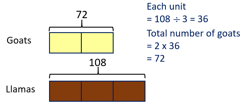
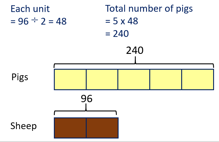
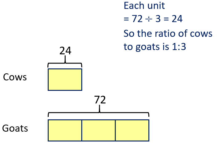
This problem is easier if you think of parts consisting of 12 animals, and the whole made of 45 parts of 12.
Animal | | Number | | Fraction |
Goats | | 72 | | 6/45 = 2/15 |
Llamas | | 108 | | 9/45 = 1/5 |
Pigs | | 240 | | 24/45 = 4/9 |
Sheep | | 96 | | 8/45 |
Cows | | 24 | | 2/45 |
Session Three
Show the student today’s starting problem on Slide 4 of the PowerPoint. Ask them to identify the important conditions in the problem:
Jessica Jones buys 60 animals at the market. She only buys cows and pigs. Cows are $120 each, three times the price of pigs. The total cost is $4 800. How many of each animal does she buy? |
- Students should recognise that pigs cost $40 each.
- Ask: Can we write the conditions algebraically?
First, the variables need defining. Number of cows might be represented by c or any other letter, and the number of pigs by a different letter, possibly p.
Second, equations can be written for the conditions.
c + p = 60 for the condition of sixty animals. - Ask: How else could this equality be expressed? E.g. c = 60 – p or p = 60 – c
- The second condition of cost is more difficult. Students may offer p = 3c to represent the cost relationship between cows and pigs. This is incorrect in two ways. P and c are used to stand for the number of each animal not the price of cows and pigs. So, the variables have changed. The relationship is incorrect as well. One pair where the price relationship holds is $12 for a cow and $4 for a pig. Putting c = 12 and p = 4 into the incorrect equation p = 3c gives 4 = 3 x 12, which is incorrect.
- Remind the students of the total legs condition from the pigs and chickens problem.
How did we express that condition?
So, 120c + 40p = 4800 represents the cost condition. - Put the students into small co-operative groups to solve the problem. Allow access to tools such as paper and pens, calculators, and computer spreadsheets. As students work, encourage them to look for similarities between Jessica’s problem and the pigs and chicken problems. The same strategies that worked for those problems; trial and improvement, diagrams, tables and algebra; should work on this problem.
- After a suitable time, gather the class to share solutions. Discuss the efficiency of the different methods. Video 4 shows a spreadsheet supported solution but other methods may be equally efficient. Students may reason that if all the animals were cows then $4800 would buy 40 cows. Exchanging one cow for three pigs keeps the cost the same but effectively increases the number of animals by two. So, ten exchanges of one cow for three pigs (a ratio) reduces the cow number to 30 and increases the pigs number to 30, which is the solution.
- The algebraic solution is also accessible, given the students’ experience in Lesson One:
c + p = 60 so p = 60 – c (total number constraint)
120c + 40p = 4800 (cost constraint)
Putting (i) into (ii) gives:
120c + 40(60 – c) = 4800
120c + 2400 – 40c= 4800
80c = 2400
C = 30
The second problem for this lesson is available on Slide 5 of the PowerPoint.
Farmer Fred goes to market. He buys 100 animals for $100. Lambs cost $10 each. Piglets cost $3 each. Chicks cost $0.50 each (50 cents). How many of each animal does he buy? |
- This is an old problem which may explain the cheap prices. It is challenging because there are only two conditions, total number and cost, but there are three unknowns, the numbers of lambs, piglets and chicks. Discuss with the students how they might simplify the search for solutions. Important observations are:
- Lambs are very expensive at $10 each, and their total cost is always a multiple of $10 ($10, $20, $30,…)
- Chicks are the cheapest animals and the number of them must be even since two of them cost a whole dollar.
- Putting those clues together can limit the search.
What is the greatest number of lambs that can be bought?
Ten lambs take up all the cost, nine lambs cost $90 and you can only buy 20 chicks with the remaining $10, eight lambs cost $80 and you can only buy 40 chicks with $20, etc.
By that thinking, the number of lambs that it is possible to buy can only be one, two, three, four or five. That makes the problem easier to solve. - Let the students work at a solution using the strategies they know from previous problems. Look for:
- Do they systematically work through possible solutions for l = 0, 1, 2, 3, 4, 5?
- Do they use diagrams and equations to support their solution finding?
- Do they use spreadsheets and adjust the variables according to the ‘number of lambs’ condition?
- Do they notice when solutions are impossible? For example, fractional or negative numbers of animals are impossible.
- Bring the class together after a suitable time to share progress towards a solution. Students can be sent away again to work in groups even if they have not found the solution after sharing.
The solution is five lambs, one piglet and 94 chicks.
Session Four
In this lesson students are encouraged to connect their strategies and knowledge of ratios to solve problems. Slide 6 of the PowerPoint poses the problem of expressing a ratio as an equation.
The ratio of pigs to sheep is 1:2. If p = number of pigs and s = number of sheep, write an equation for this relationship. |
Before asking for suggestions make a table of possible numbers for p and s:
Number of pigs (p) | Number of sheep (s) |
1 | 2 |
10 | 20 |
3 | 6 |
5 | 10 |
7 | 14 |
0 | 0 |
Students are likely to suggest two equations, s = 2p or p = 2s. Check to see which of the equations works with the table values. An important idea is that p and s refer to numbers of animals not an individual animal, pig or sheep. So, the equation s = 2p works but seems counter-intuitive with the way the ratio is said, “For every pig there are two sheep” or “There are twice as many sheep as pigs.”
- Slides Seven and Eight give two other ratios for the students to write as equations.
The ratio of goats to cows is 1:5. So c = 5g is the equation.
The ratio of horses to llamas is 2:3. So 2l = 3h is the equation. Check by putting trusted pairs of values for h and l into the equation. If h = 20 and l = 30 then the equation predicts 2 x 30 = 3 x 20 which is correct.
In each case creating a table of values helps to verify the correct equation. - Next the students work on Copymaster 3. This worksheet presents several problems in a form where ratio statements provide one of the conditions to satisfy. If students can turn the ratio statements into algebraic equations, they can use the strategies learned previously. The last problem is very difficult and designed for extension.
Solutions:
Problem One: 183 pigs
Problem Two: 84 chickens
Problem Three: 57 kids
Problem Four: 27 cows
Problem Five: $220 for the worth of the goats

Getting partial to decimals
This unit supports students to understand the place value structure of decimals and to carry out addition and subtraction with decimal numbers to three places.
The decimal system uses repeated, equal division into ten parts to create smaller units. Dividing one metre into ten equal parts creates deci-metres, a unit that is used in Europe but seldom in New Zealand. A decimetre is one tenth of a metre. If one decimetre is cut into ten equal parts, the parts are called centimetres. That is because 100 centimetres compose one metre (one tenth of one tenth equals one hundredth or 1/100). A height of 1.78 metres is a combination of 1 whole metre, 7 tenths of one metre, and 8 hundredths of one metre.
Decimal fractions underpin most of the units used in the Standard International (SI) system of measures. For example, one kilogram equals 1000 grams, so one gram is 0.001kg (one thousandth of a kilogram). One litre of water has a mass of one kilogram. Therefore, 1g is the mass of 0.001L (litre) of water, otherwise known as one millilitre. Milli is the Latin prefix for one thousandth.
There are subtle differences in the way decimals behave compared to whole numbers and reliance on whole number thinking is the key cognitive obstacle for students working with decimals. Ordering decimals is a good example. With whole numbers 7<81<657 but it is incorrect to order decimals by ‘longer is bigger’ strategies. 0.81 is greater than 0.7 but 0.657 is not greater than 0.81. Similarly, methods of calculation used with whole numbers must be changed to accommodate decimal fractions. For example, 7 + 28 = 35 but 0.7 + 0.28 ≠ 0.35. The decimal point needs to be thought of as a marker for the ones place, rather than as a ‘separator’ that keeps the whole numbers and fractions apart.
Two key concepts must be connected for students to understand decimals and how to operate on them. Whole number place value must be extended to tenths, hundredths, thousandths, and so on (following the structure of the base 10 system). This must include recognition that units are nested in other units, e.g. 2.35 has 23 tenths (23.5 tenths to be exact). Equivalent fractions are applied to compare decimals by size, e.g. 0.81 is composed of 8 tenths and 1 hundredth, since 8/10 = 80/100, 0.81 equals 81/100 (81 hundredths).
Students can be supported through the learning opportunities in this unit by differentiating the nature and complexity of the tasks, and by adapting the contexts. Ways to support students include:
The contexts for this unit are about lengths (heights). Most students find personal data interesting though caution is needed around using measurements such as body weight. Decimals occur through measurement. You might choose contexts that engage your students. For example, Census At School collected data about the weight of school bags, reaction times, and foot lengths. You might also look at populations of countries expressed as millions, e.g. 5.38 million, at distances of planets from the sun in astronomical units, at the number of gigabytes in movie downloads, or the areas of pieces of land in hectares or heights of different sportspeople. Choose contexts that engage your students' cultures and interests.
Te reo Māori vocabulary terms such as tau ā-ira (decimal number), ira ngahuru (decimal point), and uara tū (place value) could be introduced in this unit and used throughout other mathematical learning.
Session One
Students should work through Getting Partial to Fractions before starting this unit as the first activities rely on a length model developed in the earlier unit.
What will the next place to the right be? Explain why?
How many of this sized unit fit in one whole metre? What will the unit be called?
These derivations could also be modelled using decipipes. Many decipipe sets use equivalent measures i.e. one unit = 1 metre, one tenth unit = 1 decimetre, and one hundredth unit = 1 centimetre.
Use your folding skills to create decimetres. Label them as 0.1 (1 tenth) except for the last one. Make the decimetre lengths with the scissors.
Take the last decimetre and fold that into centimetres. Label them as 0.01 and cut them out.
Watch for students to:
How might we sort these data?
Make each height using metres, decimetres and centimetres, or the decipipe equivalents.
Record each height like this: 1.56m = 1 + 5 tenths + 6 hundredths.
Imagine that your group was joined ‘head to foot’ – What is your combined height?
The first challenge is to order the heights of four teenagers. Can your students correctly name the teenagers by looking at the place value structure of the decimals?
e.g. 1.8m is taller than 1.65m. By how much?
The second challenge has four aspects, including finding decimals with a given difference, and planning an ordering strategy. A key point is that ten hundredths combine to make one tenth, e.g. 1.57 + 3 hundredths = 1.6.
Session Two
In this session students explore addition and subtraction of decimals.
How high is the doorway?
How tall is Robert?
Recall that Scott Barrett is 1.98m tall? How much taller is Robert than Scott? Compare Steven Adams' height of 2.11m with Scott and Robert
Is Rufus correct? Explain.
Why does Barbara say the answer must be more than 3 metres?
How does she know?
What should the answer be?
Your task is to work out some combined heights. First try all the pairs of people you have in your group, then try the whole group combined. Use the metre, decimetre, and centimetre strips, if you need. Record the answers you get using either a number line or written algorithm.
When two heights are added what is the usual range for the sum?
Why is the sum usually 3.0 – 3.5 metres? (The average height of 11-13 year olds in New Zealand is about 1.6 metres)
Is the average different for males and females?
Session Three
In this session your students look at the two situations to which subtraction of decimals can be applied, partitioning (separating) and difference. The range of decimals is still constrained to hundredths.
Compare the proportions of the Barbie doll with the normal proportions of a female. What do you notice?
Look at the diagram of normal proportions for men and women.
What do you notice?
What will the rest of Aisla/Barbie measure? Share your strategy.
Subtraction is the most obvious strategy since part of Aisla or Barbie is removed, leaving the rest. For example, 1.76 - 0.9 = 0.86m gives the length from Aisla’s hip to the top of her head.
Measure the length from your navel to the top of your head, and subtract that length from your height. What will the difference tell you? Show your working and answers in decimals of one metre.
Session Four
In this session students expand their knowledge of the decimal system to include thousandths. The need for smaller units is inspired by a need for more accuracy. Your students will need access to strips of paper that are exactly one metre long.
How long is one half?
Some will say 50cm which is correct. Write 50/100 and ask what the fraction is referring to. Note that one half and fifty one-hundredths are equivalent fractions.
Many students know that one half equals 0.5. Performing 1 ÷ 2 = 0.5 on a calculator confirms that.
What does the five mean? (five tenths)
How long is one quarter?
What is the decimal for one quarter?
If one quarter equals 0.25 then what is the decimal for three quarters?
Session Five
In this session students apply their knowledge of decimals to three places to solve addition and subtraction problems. They investigate rainfall patterns for different locations in New Zealand then play a game that involves addition and subtraction of decimals.
Is there any pattern to the rainfall in New Zealand? (East Coast tends to be drier than West Coast)
Which locations have the highest/lowest rainfall?
How would Wellington’s annual rainfall be written in metres?
Add the rainfalls of Tauranga, Gisborne, and Napier. Give the answer in metres.
Hemi claims that the Eastern North Island gets nearly 3m of rain per year. Is he right? Explain. (It is not legitimate to add the rainfall of different locations).
“We get more than 10cm less rain than the next driest city, and half the rainfall of Auckland,” she says.
It’s all very confusing. Is she right?
Alexandra is not a city, but it gets only 0.335m of rain per year.
How much less rain does it get than Christchurch?
Extras
For further development of decimal understanding students should attempt the four e-ako modules that cover addition and subtraction of decimals using a decimat model (AS4.10, AS4.20, AS4.30, AS4.40). That is best done over four days. Each module takes around 20 minutes to complete.
Create 2.8 and Decimal Lineup can be sent home as practice games for students to play with their family.
Dear family and whānau,
This week we have been exploring decimals and how to add and subtract those numbers. We will be measuring lengths in metres, including our heights and rainfalls for different towns.
During the unit we will learn that decimals behave differently to whole numbers when we add and subtract them. However, our knowledge of whole numbers will still come in very handy.
Fitness
This unit examines regular tessellations, that is, tessellations that can be made using only one type of regular polygon, and semi-regular tessellations, where more than one type of regular polygon is involved. Students are required to investigate what properties tessellating shapes must have in order to cover the plane with no gaps or overlaps.
Tessellations are frequently found in kitchen and bathroom tiles and lino. You can see them in the pattern on carpets and decorative patterns on containers and packaging. They play a significant role in tapa cloth design and creation, and in Islamic art that features designs commonly built around star polygons. Tessellations are a neat and symmetric form of decoration. They also provide a nice application of some of the basic properties of polygons.
To be able to fully understand the concept of tessellations using regular polygons, you need to recognise their symmetry, and be able to calculate the size of their interior angles. This information is accessible to Level 4 students. In this unit, students are led through the steps needed to establish that there are only three regular polygons that tile the plane. This unit follows on from Keeping in Shape from Level 3, where regular tessellations are first discussed.
Moving on from here, the children can consider semi-regular tilings. All that they need to know here is how to sum the interior angles of various regular polygons to 360°. The rest is up to their imagination.
This unit is designed for students to learn and practise outcomes at Level 4 of mathematics in the New Zealand Curriculum. The geometric focus opens up opportunities for visual reasoning that might prove engaging for students who find numeric reasoning challenging. Here are some approaches to enabling participation.
The difficulty of tasks can be varied in many ways including:
The contexts for this unit can be adapted to suit the interests and cultural backgrounds of your students. Investigate the use of tessellation in cultural designs such as the mosaic art and architecture of the Moors, Greeks, and Persians in Europe and China and Japan in Asia. For example, tessellations are prominent in Islamic art traditions, and in tapa cloth designs from Pacific nations. Students might be fascinated by the work of Dutch artist Escher, who built his work on distorting regular polygons to create ‘life-like’ tessellation patterns. Tessellation might fit well with efforts to beautify the school environment, such as creating a class mural. Mosaic tiles can be created from fired clay, or cobblestones created from concrete.
Getting Started
Show the students a large cut out equilateral triangle. Mark the vertices (corners) of the triangle with different colours. Say, "I am going to tear off the corners of this triangle and place them around this point (draw point on board). What do you think will happen?" Students may have encountered this before but let them guess what they think will happen. Tear off the corners and place them about the point to confirm that a half turn (or 180°) is created.
If the sum of the interior angles of any triangle is the same - 180°, is it likely that the sum of the interior angles of any quadrilateral is the same? Ask them to predict what will happen if the corners of any quadrilateral are joined about a point. Have them cut out several quadrilaterals of different shapes to check their predictions. Remind them to mark the corners before tearing them off.
Once it has been found that the sum of the interior angles of any quadrilateral is 360° (they form a full turn about a point), then students can investigate the sum of interior angles of other polygons by measuring with protractors or tearing corners. You may need to model how to find the size of an angle using a protractor. The results can be captured in the table below. Encourage the students to look for a pattern to predict what the next angular sum will be.
Number of Sides
Sum of Angles °
Interior Angle of Regular Polygon
3
180
4
360
5
540
6
720
Note that for each side that is added, the sum of the interior angles increases by 180°. This can be explained by the fact that the addition of a side creates another triangle within the shape, and that each triangle has an angular sum of 180°.
What size are the interior angles of the regular figures we have just been talking about? How can we find out?
For the regular hexagon with six vertices and an angular sum of 720°, we need to divide the sum by the number of angles to find each angle size. So, since 720 ÷ 6 = 120, each interior angle in a regular hexagon is 120°.
Exploring
Use a set of pattern blocks to show how equilateral triangles tessellate. Tessellate means that they cover the plane infinitely with no gaps or overlaps. Send the students away in groups with their own set of pattern blocks, or access to an online version (search for Pattern Block Virtual Manipulative), to explore what other tessellations can be discovered using shapes from the set. You may want your students to record the tessellations using isometric dot paper.
After a period of exploration, bring the class back together to share the tessellations. Note that there are three regular tessellations that can be found, that is tessellations involving use of the same regular polygon. These regular tessellations are 3.3.3.3.3.3 (six triangles about each point or vertex), 4.4.4.4 (four squares about each vertex), and 6.6.6 (three hexagons about each vertex).
Focusing on the regular tessellations ask why it is that these patterns work without gaps or overlaps. You may need to remind the students of the angle measures they found in Getting Started. There are two key properties of the shapes involved in regular tessellations:
Note that with some vertices the arrangement is 6.3.4.4 and at others it is 6.4.4.3 if the shapes are read clockwise about each vertex.
Reflecting
There are two approaches for this depending on the ability of your students. The first way is to notice that no polygon has an interior angle greater than 180°. They are always less than this. And no polygon has an interior angle smaller than 60°(from the table.) That means that you need at least three polygons to come together at a vertex and no more than six polygons since 6 x 60° = 360°:
Only three of these are possible for regular polygons. The only tessellation by regular polygons requires an equilateral triangle, a square or a hexagon.
Dear family and whānau,
This week we have been experimenting with tessellation of the plane with polygons. In particular we have found that regular tessellations can only be made with equilateral triangles, squares and hexagons.
Regular polygons have all sides equal and all angles equal.
Figure it Out Links
Some links from the Figure It Out series which you may find useful are:
Tessellating Art
In this unit we apply our understanding of why tessellations work to form our own unique tessellating shapes. We use these shapes to create interesting pieces of art in the style of M.C. Escher, a famous Dutch artist.
This unit is built around the famous artist Maurits Cornelius Escher. Escher was born in Leeuwarden, Netherlands on June 17th, 1898. He studied at the School of Architecture and Decorative Arts in Haarlem but soon gave up architecture in favour of graphic arts at the age of 21.
All M. C. Escher works (C) Cordon Art, Baarn, the Netherlands. All rights reserved. Used by permission.
Escher is famous for two types of engravings. One of these involves impossible situations and the other is his variation on the theme of tessellations. A typical impossible situation shows four men climbing stairs. As you follow the men around and up their particular flights, you realise that they are going round and round. With regard to tessellations, Escher took a tessellation and, by adding and subtracting from the basic unit of the tessellation, turned it into a repeated picture.
There are many web-sites that explore the life and work of M.C. Escher. You can easily find one by entering his name in your search engine.
By emulating Escher and exploring tessellations in this unit, the students will gain a greater appreciation of the way that tessellations work. Hence they will see how mathematics, art and even nature interact.
Other units that refer to tessellating are Keeping in Shape, Level 3 and Fitness, Level 4. It might be useful to have done Measuring Angles, Level 3 before attempting this unit.
Students can be supported through the learning opportunities in this unit by differentiating the nature and complexity of the tasks, and by adapting the context to suit the interests, experiences, and cultural backgrounds of your students. Ways to support students include:
The difficulty of tasks can be varied in many ways including:
The contexts for this unit can be adapted to suit the interests, experiences, and cultural backgrounds of your students. For example, tessellations are prominent in Islamic art traditions, in tapa cloth designs from Pacific nations, and in Māori tukutuku panel designs.
Tessellation might fit well with efforts to beautify the school environment. Mosaic tiles can be created from fired clay, or cobblestones created from concrete or mud bricks. Once they are fired or dried they can be painted in traditional Maori patterns that reflect transformation.
Te reo Māori vocabulary terms such as rōpinepine (tessellate, tessellation), neke (translate, translation), huri (rotate, rotation), whakaata (reflect, reflection), and hangarite (symmetry, symmetrical) could be introduced in this unit and used throughout other mathematical learning.
Getting Started
We begin our exploration of tessellating art by altering squares and parallelograms.
What can you tell me about this tessellation?
Why is it a tessellation?
Which of the regular tessellations does it look like it has been made from?
Can you see how this tessellation has been made? Show us.
Look at the tessellating shape and predict how it was altered.
Will your new shape tessellate? Try it and see.
Is your altered shape symmetric? What type of symmetry does it have?
Does the new shape have to be symmetric to tessellate?
(Note: When altering a square by translating opposite sides to form a new tessellating figure, the alteration does not have to be symmetrical.)
Describe the movement of the shape as you tessellate with it? (translation or shifting)
What did you discover about altering shapes to create new shapes that also tessellate?
Why do you think it is possible to alter shapes in this way and still end up with a shape that tessellates?
Did you create any shapes that do not tessellate? Why do you think that they won’t tessellate?
Exploring
Over the next 2-3 sessions we use our imaginations to create interesting art pieces using altered tessellating shapes.
Brainstorm for ideas about what the shape could be. In the following shape the addition of an "eye" creates a fish-like shape.
Tell me about the symmetries of your shape? (reflection symmetry, rotational symmetry)
How are you generating the tessellation? (translating? rotating? reflecting?)
Why does your shape tessellate? (Encourage the students to focus on the fact that the sum of the angles at any point must equal 360 degrees)
Reflecting
In this final session we analyse tessellations and attempt to predict the processes that were used to create them.
What shape do you think has been altered?
How do you think it was altered?
Dear family and whānau,
This week we have been working on a unit that changes a square tessellation into a piece of art similar to that produced by a famous Dutch artist called Escher. At home this week we would like you to help your child transform an equilateral triangle into an interesting piece of tessellating art.
All M. C. Escher works (C) Cordon Art, Baarn, the Netherlands.
All rights reserved. Used by permission
Figure it Out Links
Some links from the Figure It Out series which you may find useful are:
What are the chances?
In this unit students investigate the link between experimental estimates of probability and theoretical probability. They also learn about short run variability and independence/dependence of events.
Simply put, probability is a measure of the likelihood of an event occurring. Just like 2.3 metres is a measure of length, 50% or 1/2 is a measure of the chance of getting heads with a single coin toss.
Probabilities range from zero to one (0-100%). An event that always occurs is certain and has a probability of 1 or 100%. An event that never occurs is impossible and has a probability of 0 or 0%.
There are two ways to estimate or calculate the probability of an event occurring. An experiment consists of trials where the event may occur. For example, a coin might be tossed 100 times and the results used to estimate the probability of heads occurring. The experimental probability is unlikely to be exactly 50% but the results will provide an approximate measure for the likelihood.
The likelihood of some events can be worked out theoretically. A model must find all the possible outcomes and identify which of the outcomes leads to the event occurring. The probability is expressed as a part-whole fraction, Number of outcomes that lead to the event/Total number of possible outcomes. In the simple case of a coin toss there are two possible outcomes, and one of those outcomes leads to the event of heads. Therefore, the probability of heads equals 1/2.
In more complex situations involving chance, models of theoretical probability become more complex. Events are independent if they do not influence each other. Tossing two separate coins involves independent events as the result from the first coin has no impact on the result from the second coin. Selecting two coloured pegs from a bag, without placing the pegs back in the bag after each turn, involves two dependent events. The result of the first peg draw affects the possible outcomes for the second peg draw.
The learning opportunities in this unit can be differentiated by providing or removing support to students and by varying the task requirements. Ways to support students include:
Tasks can be varied in many ways including:
The context for this unit can be adapted to suit the interests and cultural backgrounds of your students. Most students are captivated by games of chance and are intrigued when their expectations about fairness do not match what occurs. This unit uses contexts such as traffic lights, fish populations, horse races, and family makeup. These contexts can be adapted to others without losing integrity, such as sampling shellfish populations, or other rare animals such as kiwi or tuatara. Horse races could be replaced by waka racing. Card games are also ideal opportunities to investigate probability.
The following te reo Māori vocabulary terms could be introduced in this unit and used throughout other mathematical learning, raraunga (data), ōrau (percentage), tūponotanga (probability, chance), pāpono (event, probability), matapae (prediction), putanga (outcome), hoahoa rākau (tree diagram), tūtohi (chart/table of data), tūtohi tatau (tally chart) , auau (frequency), kauwhata porowhita (pie graph).
Session One
(Maybe the fans can explain how the game works. Perhaps show a brief highlights video from a recent game). This context could be adapted to recent sports events that are relevant and interesting to your students (e.g. Olympic sports, Rugby World Cup matches). The learning in this session could be used as the basis for independent/paired student investigations into different sports teams and matches.
What do you think a simulation is?
A simulation is an imitation of the real thing, so the game will not be real.
Discuss: What positions shoot for a goal in netball? (Goal Shoot and Goal Attack)
I have looked at a few games played between the two teams to see how accurate the goal shooters are. Here is the data.
Show them this table of results:
How many games between the two countries do you think are included in these results? Explain. (Teams usually score around 50 goals per game)
How can we compare how accurate the shooters of both teams are?
(Students need to recognise that there were different numbers of shots taken so fractions/percentages are needed. Look online for netball shooting statistics to see that percentages are used – Why? Use a calculator to find the percentages, i.e. 259 ÷ 298 = 87% and 277 ÷ 324 = 85%, and discuss rounding to the nearest percent)
What is the purpose of working out the shooting percentage?
What are the chances that this shot will be a goal?
Expect words such as likely, almost certain, probably.
Expect numbers such as three quarters (3/4), 85%, 0.8.
Let’s imagine that rolling the dice is like taking a netball shot. When a Rockets player takes a shot, the numbers 1-5 are goals, and 6 is a miss. When an Emeralds player shoots the numbers 2-6 are goals, and 1 is a miss.
Write the rules on the board:
How many games ended in a draw? In a set of 25 games around seven, eight, or nine will end in draws. There is slightly less than one third chance of a draw.
What are the ways a draw might happen? (Both teams get three goals, two goals, one goal, or no goal)
Collate the results (for example):
Do the results match our predictions? Why? Why not?
Expect students will comment that the results were unpredictable. In probability the word random is used to describe an outcome that is uncertain. However, the number of wins for Rockets and Emeralds are close.
Is a draw more likely with more shots in a game?
Is it more likely that the winning sides are more balanced with more shot games?
Students might note that the results for a small number of shots are erratic and do not appear to match the theoretical idea that both teams have the same chance of winning. This is known as short-run variability, that is, the outcomes from a short number of trials often vary from expectations. You might also discuss the difference between an outcome and an event. A win for Rockets, a win for Emeralds, and a draw are events, things that may or may not happen. Many different outcomes contribute to those events. For example, Rockets might win by their three shots all being goals with Emeralds scoring two, one, or no goals.
Session Two
A couple I know are expecting their first baby (pepe). They are not worried about which gender the baby (pepe) is, but secretly I think they want a girl.
What are their chances of getting a girl baby (pepe)?
Does anyone in the class come from a family that has two children?
What are the genders of the children in your family, starting with the first born?
Record the data you get from students.
MF FF MM FM MF MM FM FF FF MM MF
If there are not many families with two children, open the data up to other families that your students know about.
Looking at these data, what are the chances of getting two female babies in a two-child family?
How reliable do you think these data are?
Students might mention issues like a small sample size, and that the sample is drawn only from our families.
Show your students how to reset the spinner each time (Clear results) before creating the next family. Ask them to work in pairs and represent their results using a tally chart.
If you prefer you could use two coins to carry out the simulation instead of the spinner (assign a gender to each side of the coin and record the results of flipping).
What do you notice? (Same gender families are about 1/4 each and the mixed family is about 1/2)
Why do these events have different likelihoods/chances?
Students may explain that there is only one way to get MM, one way to get FF, but two ways to get a mix, MF and FM.
Which outcomes give a mixed two-child family? Circle those outcomes.
Which outcome is a Male-Male family? Circle that outcome.
Which outcome is a Female-Female family? Circle that outcome.
Note that two outcomes out of four give a mix of male and female (MF and FM). 2/4 is equivalent to ½ and 50%.
What mixes of female and male children are possible in a three-child family?
Use the spinner (or coins) to simulate having three-child families, at least 24 times.
Record your results.
Which events happen most frequently?
Which events happen least frequently?
Create a tree diagram to explain your results.
What is the probability that all the children will be female? (1/8 or 12.5%)
What is the probability that all the children will be male? (1/8 or 12.5%)
What is the probability of a two-female and one-male family? (3/8 or 37.5%)
Where do these two-female and one-male outcomes appear in the tree diagram?
How many possible outcomes result in the event of a two-female and one-male family? (Three: MFF, FMF, FFM)
Why is the probability of a two-male and one-female family the same, 3/8?
Jacob tosses two coins. Each coin has a heads side and a tales side.
“There are three possible outcomes, two heads, two tails, or head and tails,” he says.
What does Jacob think is the probability of getting two heads?
Is he correct? Explain.
Do students notice that the situation is the same as the two-child family scenario?
Session Three
In this session students explore the implications of independent and dependent events.
Who likes fish? Who likes fishing?
What species of fish/ika moana can we catch in Aotearoa?
Which species are found in fresh water?
Students might suggest species like trout (brown, rainbow), eel, bullies, etc. Most species in New Zealand lakes are introduced, usually as game fish. This learning could be linked to fish or animals that are significant to your local area, or to learning about pests or native animals (e.g. mudfish).
You might play a short video about freshwater fish. Forest and Bird has some interesting examples.
Imagine a tiny lake that has only four fish, two trout and two perch.
A scientist catches two fish out of the lake, one after the other. The second fish bites so quickly there is no time to return the first one.
What species might the two fish be?
Two Trout (T1 and T2) Two Perch (P1 and P2)
Trout-Perch (Note that four outcomes can result in this event, T1 and P1, T1 and P2, T2 and P1, and T2 and P2)
Students may mimic the probabilities from two-child families (1/4, 1/4 and 1/2).
Are the results what we expected?
Students should note that the proportions are a long way off 1/4, 1/4 and 1/2.
Have we got enough data? Do we need to trial the fish catching again?
100 trials represent a reasonable sample size.
Think about the situation. Can you create a model to explain these results? Discuss the model with your partner. Record your thinking.
How many of those outcomes result in a trout and perch combination? (8 out of 12 or 4 out of 6)
Can we express the probability of a mix, as a number? (2/3 or about 67%)
What are the probabilities of two trout and two perch being caught? (1/6 each)
What do the probabilities add up to? (2/3 + 1/6 + 1/6 =1 or 100%)
How is this situation different from the two-child family situation?
Try changing the fish in the lake using Copymaster 2.
Create different mixes of trout and perch in the lake.
What mix gives a probability of ½ that the two fish caught are the same?
What mix gives a probability of 4/10 that the two fish caught are the same?
Try different mixes and work out the probabilities.
Session Four
In this session, students explore a situation in which the probability of each outcome is not equal. To solve the problem, students need to adjust their method of finding all the possible outcomes to balance the different likelihoods.
What fraction of the time are the lights on each colour?
1/2 on red, 1/3 on green, and 1/6 on orange.
How might we simulate Luciana travelling through two sets of traffic lights?
Students might suggest creating a spinner and spinning twice. There are other ways to simulate traffic lights, such as using a standard dice:
1-3 represents a ‘stop’ signal, 4-5 represents a ‘go’ signal, and 6 represents a ‘lights changing’ signal.
Talk about how you will organise the data you get from your simulation trials.
What events might occur when Luciana goes through two sets of lights?
(Apart from saying she might have a crash, students might suggest that she stops zero, one or two times)
Which event do you think is most likely? Why?
Given that Luciana must stop 4/6 or 2/3 of the time at a given set of lights, students should forecast that there will be a lot of stopping.
What do you notice?
(The fractions for two stops and one stop are similar. Theoretically both probabilities are the same at p = 4/9.)
Luciana gets through both sets of lights only 11% of the time. What fraction is that? (11/100 or about 1/9)
Expect students to conjecture that there is more chance of having to stop at a set of lights, so both options, stopping once, or twice, are more common.
What does this table show?
What does the different shading of areas represent? (Dark grey is the ‘stop at both lights’ area, mid-grey is the ‘stop at one light’ area, and light grey is the ‘no stop’ area)
Which area is the greatest? (Dark and mid-grey have the same area, 16/36)
What do the areas tell you about the chances of stopping?
Session Five
In this lesson we conclude the unit with a game that involves probability.
Does that seem fair?
Which horse has the best chance of winning? Why?
Students should comment that the horses that have the furthest to go move more often and the horses with the least distance to go move least often.
Why do some horses move more often than others?
How could we find all the possible outcomes, when two dice are rolled, and we find the difference?
Remember that we have used tree diagrams, tables, and networks before in this unit.
Are those methods useful here too?
Is 1 on the first dice and 5 on the second dice the same outcome as 5 on the first dice and 1 on the second dice? (No. They are different outcomes, a bit like Trout 1 and Perch 2 being different to Trout 2 and Perch 1)
How many different outcomes are there? (36 possible outcomes)
How many outcomes give the event of Horse Zero moving? (Six, (1,1), (2, 2), (3, 3), (4, 4), (5, 5) and (6, 6).
The table shows the differences produced from the set of outcomes.
What patterns can you see in the table? (Students might note the diagonal arrangement of cells with the same differences)
Which horse has the best chance of moving? How do you know?
Can you find the probability of Horse One moving on a single throw? (10/36 ≈ 28%)
Is the game fair? Does each horse have an equal chance of winning the race?
Students might match up the probability of each horse moving on a single throw and the number of steps the horse needs to win.
The table shows that the distances balance the probabilities well except for Horse Six that has no chance of moving.
Assessment
Evaluate students’ understanding of probability using the multiplication basic facts game called Multi-Bet. You will need two dice labelled 4, 5, 6, 7, 8, 9, counters, and a game board for each group of players. In this scenario the students are placed in the shoes of Risky Betts, the Casino owner, who has to determine the payouts for the game.
Each player starts with ten counters (their loot!).
They place bets in the following way:
The winning number is determined by tossing the two dice and multiplying the numbers that show (e.g. 4 x 6 = 24).
If the winning number is not in those selected by a player, then the casino takes all the counters.
If the winning number is one of those chosen by some students, then the casino must pay out. How much should the Casino pay out for each type of bet?
The odds must be enticing to the players yet ensure in the long run that the casino makes a profit.
Note that there are twenty products on the board in total so that a bet covering four numbers has a four out of twenty (4/20 = 1/5) chance of being successful. The casino will want to offer odds of less than 5:1 if they are to make money in the long run.
Some students may note that there are more ways for some numbers to occur than for others. For example, thirty-six can occur in three ways (4,9), (6,6), and (9,4), whereas forty-nine can only occur in one way (7,7).
Teachers: Provide Copymaster 5 to each child for them to take home.
Dear parents and whānau,
This week in maths we have been exploring probability in interesting ways. Probability is how we measure the likelihood of an event occurring.
Here is a problem to solve with your child.
Each time you buy a meal at Buns Burgers you get a card drawn from the Free Burger Box. The card will show the left, centre, or right side of a hamburger. When you have collected three cards that make a whole hamburger you can exchange it for the real thing!
Assuming that Buns Burgers put the same number of each card in their Free Burger Box to start with, and each time you get a card it is purely by chance (random), how many meals will you need to buy to get a free hamburger?
Enjoy investigating this probability problem with your child. You might both be surprised.
Down on the farm
The unit is designed as a simple introduction to systems of linear equations. Students solve problems in which they meet two constraints to find a single solution. Both constraints can be expressed as linear equations.
Systems of equations are extremely useful for modelling real world situations. Often two or more conditions exist in a situation that must be satisfied. We can often express conditions using representations such as tables, graphs and equations. These representations provide powerful tools for solving problems.
As an example, consider simultaneously meeting these two conditions:
Condition (i) can be represented by the following table, graph and equation.
c = 2p or p = c/2 where p represents the number of pigs and c the number of chickens.
Condition (ii) can be represented in the same ways.
c + p = 90 or c = 90 – p or p = 90 – c
Satisfying both conditions involves finding values for the number of pigs and number of chickens that work. In table form this involves searching for a common pair in both tables. In graph form this involves finding an intersection of both lines.
An algebraic method is to solve the two equations simultaneously. There are different ways to do this. Here is a substitution method:
Putting 2p in for c in equation (ii) gives:
2p + p = 90 so 3p = 90 and p = 30.
Since c + p = 90, c must equal 60.
The problems in this unit involve using representations to meet common conditions.
Specific Teaching Points
Representing relations in algebraic equations involves two important and connected types of knowledge, related to the language conventions (semiotics), and to the nature of variables. When we write c = 2p, or c = 90 – p + 2 the equations are meaningless to anyone else unless we clearly define what the variables, c and p, represent. Note that both c and p refer to quantities that vary and are not fixed objects, such as a chicken or a pig. Quantities are a combination of count and measurement unit. In this case c expresses many animals. Animals are the unit in this problem. 2p means the number of pigs multiplied by two, not twenty-something.
Semiotics, the meaning of symbols and signs, is central to algebra. Transfer between semiotic forms is difficult at times. For example, a statement such as “there are twice as many chickens and pigs” seems innocuous and it is easy to generate a table of values that satisfy the statement. However, recording the statement as an algebraic equation requires a student to accept letters as variables, not as objects that can be counted. 2p = c or c = 2p is correct but appears ordinally different to the spoken form. Some spoken languages are more consistent with algebra and would express the relation as “To get the number of chickens multiply the number of pigs by two.”
Working with variables also requires acceptance of lack of closure, that is thinking with symbols (c and p in this case) without specifically knowing the values they hold. For example, knowing that c = 2p can be substituted into c + p = 90 while conserving its structure, irrespective of whatever the value of c or p, is itself a generalisation.
The equals sign represents a statement of ‘transitive balance’ meaning that the balance is conserved if equivalent operations are performed on both sides of the equation. Knowledge of which operations conserve equality and those which disrupt it are important generalisations about the properties of numbers under those operations, e.g. distributive property of multiplication.
Students can be supported through the learning opportunities in this unit by differentiating the nature and complexity of the tasks, and by adapting the contexts. Ways to support students include:
Task can be varied in many ways including:
The contexts for this unit can be adapted to suit the interests and cultural backgrounds of your students. Animals on the farm provide the contexts for all problems in the unit and appeal to a range of students. Other contexts can also be used, such as buying items at a shop, e.g. socks at $3 per pair and hats at $12 each. Catering at a marae or tulaga fale provides a useful context around managing a budget while still providing ample food for manuhiri (visitors). People in an extended whānau also provides an interesting context, with variables such as the number of adults and children.
Te reo Māori vocabulary terms such as ōrite (equal), kīanga taurangi (algebraic expression), kīanga ōrite (equivalent expression) and whārite rārangi (linear equation) could be introduced in this unit and used throughout other mathematical learning.
Prior Experience
It is anticipated that students at Level 4 and 5 understand, and are proficient with, multiplicative thinking. Students are expected to know about simple ratios though this unit reintroduces some key ideas. Some proficiency at solving linear equations would be beneficial, so working through the units on linear algebra before this unit would be helpful.
Session One
Begin with this new version of a very old problem. The problem solving pathway in e-ako maths includes a version of this problem called "Sheep and chickens". This might be used as an extension task for students who enjoy the algebraic equation approach.
On Mr MacDonald’s farm there are only pigs and chickens.
He counts 24 heads and 80 legs.
How many of each kind of animal is there?
After discussing important conditions in the problem, encourage the students to work in small co-operative groups. Allow access to supportive tools such as calculators and computers. Recording on paper will be important.


Look for the following common approaches:
Trial and improvement
This approach typically involves choosing a pair of possible values for the number of pigs and chickens, and making alterations until the other condition is met. For example, 12 pigs and 12 chickens might be tried. This assumption meets the number of heads condition but 4 x 12 + 2 x 12 = 72. So that pair of values fails the number of legs condition. However, systematic adjustment of increasing the number of pigs and reducing the number of chickens will eventually give the answer. Note that this strategy is very protracted if the numbers involved are large.
Figurative diagram
Students using this strategy often begin with numbers of pigs and chickens that satisfy the number of heads condition, though sometimes they draw 48 animals of one kind. Some students draw figures that satisfy the number of legs condition. It is important that the drawings are symbolic and not literal (i.e. not life-like pigs or chickens) for two reasons. Life-like drawings are time consuming and indicate that the farmyard context assumes more importance than the conditions of the problem. A drawing might look like this, with 12 pigs and 12 chickens:
Chickens can easily be turned into pigs by adding two extra legs until a solution is found that meets the number of legs condition.
Making a table
Often students’ approach the problem using trial and error (rather than improvement). They try combinations of pigs and chickens in an unsystematic way. A table helps them to organise their data but also allows for noticing of patterns that otherwise are missed.
An example of a table based strategy is given below:
The table can be extended until a solution is found. Note that use of a spreadsheet makes this strategy highly efficient.
Equations
This strategy is unusual for students at Level 4 unless they have exposure to writing and solving linear equations (link to first algebra learning object unit). First, students need to identify the variables in this problem. While it makes sense to use p and c as symbols, it is very important that students regard these as variables not fixed objects. P is not a pig nor is c a chicken. P represents possible numbers of pigs and c possible numbers of chickens.
Second, students need to write the conditions using these variables. Conventions are involved here, notably that 4p means 4 x p and 2c means 2 x c, and equals means a state of balance or sameness.
Third, solving for p or c involves trusting that these variables can remain ‘unclosed’ and conserved under a sequence of steps. This is a significant shift from arithmetic thinking which aims to ‘close’ the answer as immediately as possible.
Equation (i) can be reorganised as p = 24 – c or c = 24 – p. Either of these equalities can be substituted into equation (ii) so the equation is in one variable:
4(24 – c) + 2c = 80 or 4p + 2(24 – p) = 80
Discussion
What kind of problem is this?
You want students to say that the problem involves variables, numbers of pigs and chickens. It also involves two constraints (restrictions) that must both be met for the problem to be solved.
Solutions:
The "Sheep and chickens" problem solving e-ako provides guidance to developing a general algebraic solution to the pigs and chicken problem.
Session Two
Introduce the next farmyard problem using slide 2 of the PowerPoint.
On Young Maree MacDonald’s farm the ratio of pigs to sheep to chickens is 2:3:5.
Maree has 640 animals in total.
How many of each kind of animal are there?
Solutions:
Problem One
Problem Two
Problem Three
Problem Four
This problem is easier if you think of parts consisting of 12 animals, and the whole made of 45 parts of 12.
Session Three
Show the student today’s starting problem on Slide 4 of the PowerPoint. Ask them to identify the important conditions in the problem:
Jessica Jones buys 60 animals at the market. She only buys cows and pigs.
Cows are $120 each, three times the price of pigs.
The total cost is $4 800.
How many of each animal does she buy?
First, the variables need defining. Number of cows might be represented by c or any other letter, and the number of pigs by a different letter, possibly p.
Second, equations can be written for the conditions.
c + p = 60 for the condition of sixty animals.
How did we express that condition?
So, 120c + 40p = 4800 represents the cost condition.
c + p = 60 so p = 60 – c (total number constraint)
120c + 40p = 4800 (cost constraint)
Putting (i) into (ii) gives:
120c + 40(60 – c) = 4800
120c + 2400 – 40c= 4800
80c = 2400
C = 30
The second problem for this lesson is available on Slide 5 of the PowerPoint.
Farmer Fred goes to market.
He buys 100 animals for $100.
Lambs cost $10 each.
Piglets cost $3 each.
Chicks cost $0.50 each (50 cents).
How many of each animal does he buy?
What is the greatest number of lambs that can be bought?
Ten lambs take up all the cost, nine lambs cost $90 and you can only buy 20 chicks with the remaining $10, eight lambs cost $80 and you can only buy 40 chicks with $20, etc.
By that thinking, the number of lambs that it is possible to buy can only be one, two, three, four or five. That makes the problem easier to solve.
The solution is five lambs, one piglet and 94 chicks.
Session Four
In this lesson students are encouraged to connect their strategies and knowledge of ratios to solve problems. Slide 6 of the PowerPoint poses the problem of expressing a ratio as an equation.
The ratio of pigs to sheep is 1:2.
If p = number of pigs and s = number of sheep, write an equation for this relationship.
Before asking for suggestions make a table of possible numbers for p and s:
Students are likely to suggest two equations, s = 2p or p = 2s. Check to see which of the equations works with the table values. An important idea is that p and s refer to numbers of animals not an individual animal, pig or sheep. So, the equation s = 2p works but seems counter-intuitive with the way the ratio is said, “For every pig there are two sheep” or “There are twice as many sheep as pigs.”
The ratio of goats to cows is 1:5. So c = 5g is the equation.
The ratio of horses to llamas is 2:3. So 2l = 3h is the equation. Check by putting trusted pairs of values for h and l into the equation. If h = 20 and l = 30 then the equation predicts 2 x 30 = 3 x 20 which is correct.
In each case creating a table of values helps to verify the correct equation.
Solutions:
Matariki - Level 4
This unit explores a variety of mathematical ideas, at Level 4 of the New Zealand Curriculum, in the context of Matariki. Matariki is a significant event in the New Zealand calendar and is celebrated in many schools. Matariki is an opportunity to engage in activities such as storytelling, astronomy, song, dance, and visual arts that have potential to enrich students’ mathematical experiences in meaningful contexts. New Year is also a chance to honour our ancestors, show care for our natural environment, and celebrate our bi-cultural and multicultural heritage.
Session One
Session Two
Session Three
Session Four
This is an integrated unit which covers several important mathematical ideas. A summary of these ideas is discussed below.
Rotation is a transformation. A rotation is a turn that can be described as an angle about a given point and a direction of that turn. For example, Figure A has the Matariki cluster of stars in its most easily recognised position. Figure B shows the same cluster turned 90° clockwise.
Mathematically we are interested in the features of the figure that stay consistent as it is rotated. These features allow us to spot the cluster however it is orientated. Distances between stars (as we see them) stay the same as does their position relative to each other. A trapezium connecting four stars will stay the same shape as the figure rotates.
Sessions one and three deal with relationships between variables. Variables are changeable quantities, for example, as year changes so does the date of Matariki. Associating changes in variables is an important idea in mathematics as it is the foundation of functions. Relationships can be represented in a variety of ways, including tables, graphs and rules. At level 4 students are not expected to generate formal algebraic notation for their rules, although many students will be capable of, and interested in, doing so. For example, a tukutuku panel might grow like this:
Each kaho (horizontal rod) has three tuinga (cross-stitches) so the pattern is easy. The data could be organised in a table or a graph.
The number of tuinga increases by three for each extra kaho so the relation is linear. The graph shows points of a straight line. Rules for the pattern take two forms, recursive and direct or function. Recursive rules tell what is done to one term to get the next, in this case “add three”. A direct rule states how to get the value of one variable from the value of the other, in this case ‘multiply by three’. Direct rules tend to be more powerful than recursive rules though they can be hard to find for some patterns.
Session four involves percentages as operators. That means the percentages are used to scale (shrink or increase) the lengths of a template. Suppose we had a simple template like this. You need to put a mark 60% along the line.
The location of the 60% mark is dependent on the length of the whole line (100%). If the space between 0 and 100% is 30cm than the 60% mark is at 18cm (30 x 60 = 18). If the line is 40cm long the 60% mark is at 24cm. Useful strategies to find a percentage mark are to use 10% as a unit, or find the unit rate (i.e. what 1% is). 10% is found easily by dividing the length by ten and the unit rate is found by dividing the length by 100.
This unit is an integrated unit aimed at outcomes for Level 4 of the New Zealand Curriculum. As such, the activities range across the strands. All activities can be adapted to cater for the strengths and interests of students in your class. Ways to differentiate instruction might include:
Although the context of Matariki should be engaging and relevant for the majority of your learners, it may be appropriate to frame the learning in these sessions around another significant time of year (e.g. Chinese New Year, Samoan language week). You might ask students to share how New Year is celebrated in their culture and at what time of the year it occurs. Consider why our calendar New Year happens in the middle of summer, rather than winter, due to importing the calendar from the Northern Hemisphere. This context offers opportunities to make links between home and school. Make links to local and national Matariki celebrations. Consider asking family and community members to help with the different lessons. For example, members of your local marae, or a local kaumatua, may be able to share local stories and traditions of matariki with your class.
Te reo Māori language is embedded throughout this unit. Relevant mathematical vocabulary that could be introduced in this unit and used throughout other learning include tātai (calculate, calculation), huri (rotate, rotation), whakaata (reflect, reflection), neke (translate, translation, move), ture (rule), kauwhata (graph), tūtohi (table of data, chart), raraunga (data), koki (angle), taurangi (variable), putu (degree - angle and temperature), and maramataka (calendar).
Prior Experience
This unit is targeted at Level 4 so students are expected to have experience at Level 3 including:
Session One
In this session students investigate some of the mathematics of astronomy associated with the rising of Matariki. They learn to recognise the cluster of stars irrespective of orientation. They also learn where to look for the stars at the beginning of Matariki and how the date of the New Year is determined.
Use PowerPoint 1 to organise the lesson.
Matariki is a cluster that wanders the skies in relation to other star formations. For eleven months of the year it is visible as it wanders. In early May it disappears below the horizon and reappears close to the horizon in late May/Early June. The ‘rising of Matariki’ refers to its appearance above the horizon just before dawn. That is why it was used as a consistent marker to determine the New Year. So the first new moon following the ‘rising of Matariki’ is when the New Year begins, but celebrations occur in the last quarter of the lunar cycle before.
There are seven stars in the cluster visible to the naked eye, though another two stars can be seen by some with keen eyesight or with binoculars. As a cluster, the seven stars stay in the same formation like a squadron of stunt pilots. However, the cluster appears facing different directions at different times which can make it hard to spot.
The site will show the quarters of the lunar cycle like this:
You might ask the students to graph the relations, preferably using Excel or another app. The graph reveals a cycle like this that might predict future and previous dates for Matariki. The lines in this graph show the cycle even though the points are discrete (individual). The cycle is erratic, unlike a tide timetable or the pattern of seasons, because the timing of Matariki is dependent on two different patterns. The star cluster varies in the date it first rises each year, and the lunar cycle of 29.5 days does not match our calendar months.
Session Two
In this session students investigate the significance of Matariki as a time of remembering ancestors. Ask students to choose an ancestor of their own who has passed in the last year or select a famous New Zealander from an online database. They look at data about the deceased, particularly the nature of the contribution the ancestor has made to the lives of others.
Dr Mātāmua shows how the star Matariki is at the bow of the great canoe Te Waka o Rangi. The rising of Matariki signals a time of letting go of the dead from the year before so their souls can be gathered in the trawling net by Taramainuku who casts them into the heavens. In that way our ancestors become stars.
Ask, “Why does it say biological whakapapa?” Children do not always live with their parents and sometimes adults find new partners. So the problem has been simplified. Some children have brothers and sisters, and cousins. Great Aunts and Uncles are also referred to as tīpuna.
So the total number of ancestors in a biological whakapapa is 1023 after ten generations.
These numbers are powers of two and can be written in index notation, e.g. 32 = 25. Note that 25 can be written as 2 x 2 x 2 x 2 x 2 (two multiplied by itself five times).
Students might notice that the Column C numbers are one less than double Column B, e.g. 1023 = 2 x 512 – 1.
The result is surprising as it only takes only 37 generations to get 137,438,953,471 ancestors. Note that you will need to custom format the cells to take large numbers before you fill down the table columns. If each generation is 25 years apart then there are 4 generations in each century.
1023 is about 1000 so 100 000 000 000 ÷ 1023 ≈ 100 000 000 (one hundred million)
Students should create categories like family, sport, arts, leadership, business, education, to sort the people into. The person might belong in several categories. For example, Henare might have been a politician as well as a leader.
Session Three
In this session students follow the connection of Matariki as a time to honour the dead and the responsibility of the living to strive for excellence. Matariki occurs in the middle of winter. Traditionally this was a time when adequate food was stored and whānau engaged in cultural pursuits like story-telling, games, creating art works, and singing. So it is appropriate for students to learn about the mathematics of tukutuku panels that adorn the wall of wharenui (meeting houses) of marae. Students look at a traditional design called kaokao. Toothpicks could be for students to communicate and refine their thinking around patterns and rules. Use PowerPoint 3 to organise the lesson.
"Take two off the number of kaho, multiply the answer by four, then add two” can be written as , where t is the number of tuinga and a is the number of kaho.
In general her rule is, “Take one of the kaho number and multiply it by two. Multiply that answer by two then subtract two” or 2[2(k-1)]-2=t.
For 18 kaho Kahu will make 18 x 4 = 72 tuinga, then subtract six to get 66 tuinga. In general his rule is “Multiply the kaho number by four then subtract six” or 4k-6=t.
Session Four
Matariki was traditionally a time when kites were flown. Some iwi believe that flying kites helps us to get closer to our ancestors whose souls are embodied as stars in the sky. In previous times kites were made from everyday materials, toetoe, raupō and harakeke (flax).
This YouTube video shows examples of traditional manu tukutuku (kites):
Dear parents and whānau,
Our next mathematics unit is based on Matariki in recognition of the celebration of the Māori New Year. We will investigate mathematics in the astronomy of Matariki, how the date is decided and how to recognise the cluster of stars in the dawn sky.
We will also learn about the significance of whakapapa, our family tree, and the mathematics of our descendants as we go back generations. A famous tukutuku design will help us learn some algebra and we will finish off using percentages to build kites to fly at the Matariki celebrations.