This unit teaches students to identify linear relationships and solve linear equations in context.
- Identify and find values for variables in context.
- Identify linear relationships in context.
- Represent linear relationships using tables, graphs and simple linear equations.
- Draw strip diagrams to represent linear equations.
- Solve simple linear equations and interpret the answers in context.
Algebra started with the need to solve problems. Al Khwarizmi, a Persian mathematician, was arguably the first person to represent linear and quadratic problems in symbolic form, and solve the problems by processes of ‘restoration’, i.e., equivalent operations that conserved equality. In fact, the word for algebra comes from the Arabic word for restoration.
It is fitting then that modern approaches to algebra focus on the thinking that underpins the symbolic systems. Algebraic thinking is concerned with generalisation. Letters, words, tables, graphs, networks, etc., are cultural tools that enable us to represent, then think with, those generalisations. With representational tools we are capable of ‘amplified cognition’ in that we can anticipate results that would never be possible if we relied solely on the physical environment, and on our limited capacity to process ideas just mentally.
Generalisation begins with noticing patterns and structures. A pattern is a consistency, that is something that occurs in a predictable way. It is the ‘what’ of algebraic thinking. Structure is about the organisation of patterns. It is the ‘how’ and sometimes the ‘why’ of generalisation. From noticing pattern and structure, we develop properties. For example, early counting involves pattern and structure. The ‘fourness’ of a collection comes from noticing sameness among collections of four, irrespective of the size, colour, texture of the objects. Structure of counting involves ideas like the order of counting the objects doesn’t matter.
Specific Teaching Points
In upper primary school, learning experiences for algebraic thinking typically begin with patterns. Usually these patterns are spatial and may be connected to some meaningful life context, though number patterns are also rich in opportunity. Patterns involve variables, that is features, some of which can be quantified. For example, consider this simple spatial pattern.
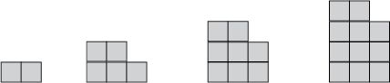
Among the variables we might discern that the ‘tower’ has height and each ‘tower’ is made of some number of squares. Height and number of cubes may not be the only variables, just those we notice. Variables change, that is height varies and so does the number of squares in the ‘tower’. We might try to find a relation between the variables, describe and represent that relation, and use it to predict how the pattern grows beyond what we can see. Then we are thinking of the properties and representations in a sophisticated way.
During this process, it is likely we will need to systematically organise the data from the pattern. A table of values is a productive, generic strategy that allows us to represent patterns, as demonstrated below:

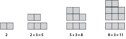
The danger in moving to an organised numeric strategy (i.e. a table) too early is that it may negate what we can ‘see’ in the pattern visually. Noticing and reasoning may be inductive, that is tied to the incremental change of the figures. For example:
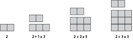
Noticing and reasoning can also be abductive, that is based on the structure of one example.
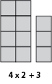
Noticing and reasoning can be deductive, that is based on making assumptions about structure and reasoning with the assumptions. For example, we might assume that the tower is composed of an array of something multiplied by three plus two.
From the assumptions we might deduce the appearance of towers much further on in the sequence, e.g. A tower 100 high will contain 2 + 99 x 3 squares. Ways of ‘seeing’ the pattern are manifest in relations within the table of values. For example, inductive thinking leads to seeing the values in the bottom row increasing by three each time. Abductive reasoning might support seeing this relation in the table:
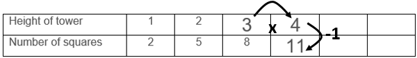
Representing the relation as an algebraic equation involves two important and connected types of knowledge, related to the language conventions (semiotics), and to the nature of variables. We might write s = 3h – 1, or s = 3(h - 1) + 2, or s = 2h + (h – 1), depending on what we notice. The equations are meaningless to anyone else unless we clearly define what the variables, s and h, represent. Note that both and s refer to quantities that vary and are not fixed objects, such as houses or towers. Quantities are a combination of count and measurement unit. In this case h expresses unit lengths in height, and s refers to an area of squares. 3h means h multiplied by three, not thirty-something, and 3(h - 1) means that one is subtracted from h before the multiplication by three occurs. Working with variables requires acceptance of lack of closure, that is thinking with an object (h in this case) without specifically knowing what it is. For example, knowing that 3(h – 1) = 3h – 3 is true, irrespective of whatever the value of h, is itself a generalisation. The equals sign represents a statement of ‘transitive balance’ meaning that the balance is conserved if equivalent operations are performed on both sides of the equation. Knowledge of which operations conserve equality and those which disrupt it are important generalisations about the properties of numbers under those operations, e.g., distributive property of multiplication.
This unit specifically deals with relations that are linear. The first sign of linearity is that there is constant difference in the increase or decrease of one variable, as the value of the other increases by one. In the table above the number of squares increases by three as height increases by one.
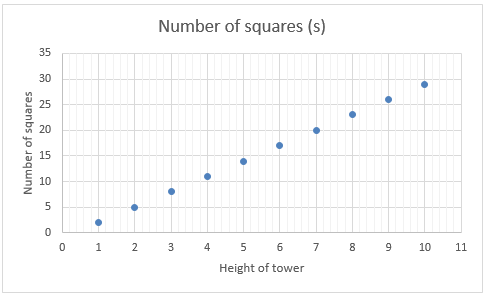
Note that this graph shows a relation, not a function, since the values of variables are discrete, not continuous. There are some important connections between features of the algebraic equation, the table and the graph of a linear relation. Constant difference is represented by the coefficient of the independent variable (s = 3h -1 in this case), differences of three in the bottom values of the table, and a slope of three (change in s for every unit change in h). The constant in the equation (- 1) is reflected in the table by a need to adjust the value of 3h by subtracting one to get the value of s, and reflected in the graph as a downward translation (shift), of the graph for s = 3h, by one unit. This results in the intercept of the graph with the s axis being (0, -1), not the origin (0, 0).
Simple linear equations occur when the value of one variable in a relation or function is set and the other must be found. For example, with the tower problem this problem might be posed; “A tower in the pattern has 98 squares. How high is the tower?” Depending on the equation used to represent the relation, this problem can be expressed as 3h – 1 = 98, 3(h – 1) + 2 = 98 or 2h + (h – 1) = 98. Linear equations with the variable on both sides occur when two conditions are equalised. An example might be, “Both Lilly and Todd look at the same tower. Lilly notices that the number of squares in the tower is three times the height less one. Todd notices that the number of squares is two times the height plus 18. How tall is the tower?” This problem can be written as 3h – 1 = 2h + 18.
The learning opportunities in this unit can be differentiated by providing or removing support to students and by varying the task requirements. Ways to differentiate include:
- using a linear model to develop the concepts of variable, as represented by a letter, and constant, as represented by a number
- developing the use of tables and graphs to organise data from a situation and look for patterns
- working with digital tools, including spreadsheets and graphing application, to develop rule seeking and equation forming
- explicitly teaching the conventions of the same operation applied to both sides of an equation. Discuss the concept of equality as ‘transitive balance’ and ask students to record steps systematically
- using the four progressive versions of Visual Algebra to differentiate the challenge for students.
The contexts for this unit include Maia Moa, working for money, ropes for gymnastics, swimming, stacking supermarket trolleys, and video games. Those contexts will appeal to most students. Use other contexts relevant to your students, in which there is a constant difference between consecutive terms (linear relationships). For example, the coach takes his car that holds three extra players. All the other players must travel on vans, seven players to a van.
Te reo Maori vocabulary terms such as wharite rarangi (linear equation), kauwhata (graph) and tau whakarea (multiplier) could be introduced in this unit and used throughout other mathematical learning.
- Access to the two digital learning objects:
- Interactive whiteboard or data projector so students can see videos and PowerPoints
- Plastic cubes or square tiles
- Access to Excel or a similar spreadsheet program
- PowerPoint 1
- PowerPoint 2
- PowerPoint 3
- PowerPoint 4
- Video 2A
- Video 2B
- Video 2C
- Video 2D
- Video 2E
- Video 2F
- Copymaster 1
- Copymaster 2
Prior Experience
It is anticipated that students at Level 4 understand, and are proficient with, multiplicative thinking. However, the tasks in this unit are also accessible for students whose preference is additive thinking. In fact, the experiences may prompt a move towards multiplicative thinking.
Session One: Maia the Moa
In this session students are shown a spatial growth pattern for a moa made from square tiles. As Maia the moa ages she grows in her legs, body and neck while her feet and head remain constant. Session One is driven using PowerPoint 1. The approach is to structure one example of the pattern then transfer that structure to other members of the pattern.
- Show the students Slide One. Aim to identify features of the pattern that might become variables. Ask: What do you notice about this figure?
Students might notice different features such as colour, height, width, age, total number of squares, etc. - Ask: Is there an easy way to count the number of squares that Maia is made of?
- Give students a while to structure their counting then ask them to share their method with others. Building a model of Maia at age three years with connecting cubes allows students to experiment with ways to partition the model. Encourage them to express their counting method as an expression. Use these videos to show examples of how to do this, but only if needed:
- Ask students to apply their counting structures to Maia at age two years (Slide Two). Ask them to record expressions for their counting strategy and compare them to what they recorded for year four.
- Ask: What changes and what stays the same in your expressions?
For example, from Casey’s method these two expressions emerge:
4 + 2 x 3 + 2 (Age two) 6 + 2 x 5 + 2 (Age four)
The ‘+ 2’ is constant and ‘2 x’ is present in both expressions. The other numbers vary. - Ask: What will your expression for Maia at age three years look like? Write the expression then check it by drawing a picture of Maia at age three (See Slide 3).
- Ask students to show where the parts of their expressions come from in the picture. For Casey’s method the expression is 5 + 2 x 4 + 2. Slide 4 shows how parts of the diagram can be linked to parts of the expression. Look at the strategies of the students.
Are their strategies based on induction? That is sequential processing. For example, 4 , ? , 6, so ? = 5, and 2 x 3, 2 x ?, 2 x 5, so ? = 4. - Are their strategies based on deduction? That is reasoning about the structure of any term. For example, the first number is two more than the age, and the multiplier of two is one more than the age. So, for y = 3 Casey’s expression is 5 + 2 x 4 + 2.
- Pose this problem for students to explore individually or in small co-operative groups:
Imagine that Maia celebrates her twentieth birthday.
How many squares will she be made of?
Find a way to predict the number of squares that Maia is made of for any age in years? - Allow students plenty of time to explore the problem. Look for the following:
- Do the students record the data systematically? For example, if they draw Maia at age five years. Are their structural counting methods consistent? Is their recording in sequence?
- Do students use inductive methods? For example, Maia increases by three squares each year.
- Do students use deductive methods? For example, applying Casey’s method Maia should be (20 + 2) + 2 x (20 + 1) + 2 on her twentieth birthday.
- How do students express their general rules? Do they use words?, e.g., “I take the age and add two to it to get the first number.....” or do they attempt to symbolise their rules, e.g. Next number = number before + 3.
- Bring the class together to discuss their methods with emphasis on the points above. Acknowledge the legitimacy of inductive methods but also highlight the power of deductive methods. Use questions like, “Which strategy would be better for finding out about Maia at 100 years of age?”
Session Two
This session builds on the Maia the moa, pattern to represent the relation between age and number of squares using a table, a graph and an equation. Features of these representations are connected through looking at the effect of changing the original spatial pattern with focussed variation.
- Open Microsoft Excel, Google Sheets, or a similar spreadsheet program and create a blank workbook. You may need to have Slide 3 of PowerPoint 1 available for source data. Ask one of the students to set up a table like this:
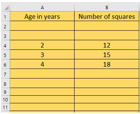
- Ask students what they notice about the table.
Some may notice missing values in the Age column, particularly the ages 0, and 1. Others may notice that the number of squares are all multiples of three. They may express this idea inductively, “The number of squares goes up by three.”
How can we continue the table to get more values? - Induction can be used to ‘fill down’ the values in both columns but deductive rules across the columns are more sophisticated. Video 2A shows how to create values by filling down. Video 2B is about using formulae across the columns. The videos can be stopped at any point for discussion. Video 2B goes straight to the most efficient rule but students could enter the rules they developed in Lesson One.
- Ask: Can you use Excel to show that your rule from yesterday works?
- Next a graph is created from the table of values. Video 2C shows how to do this. Ask the students to create their own graph of Maia’s growth patterns and record some features that they notice.
Why are the points in a line? (This tell us that the relation is linear)
How steep is the line?
Note (0, 6) represents Maia’s situation upon hatching.
Where does it cross the s axis?
Why does it cross there? - PowerPoint 2 offers three scenarios in which Maia’s shape is changed in some way. The reason for doing this is to connect features of the table and graph with the spatial pattern. For each scenario students may need to draw the progression of each pattern back until Maia hatches. That will lead to a table of values that can be graphed. Video 2D shows what happens when the original Maia growth pattern is altered by a constant, - 1 for losing her foot and + 2 for gaining a backpack. Video 2E and Video 2F show the effect of changing the coefficient (multiplier) of a, in that the slope of the graph alters from three to four. Copymaster 1 provides printable versions and the start of a table for each.
Session Three
- Remind the students of the rule that was entered into your spreadsheet to create the pattern in the Number of squares column for Maia’s original growth pattern (e.g. =(A2+2)*3).
What does A# represent? (Maia’s age in years, a). So instead of A# we could write = (a + 2) x 3 or = 3(a + 2).
What does this expression tell us? (The number of squares Maia is made up of). So we could write s = 3(a + 2). - Show the students PowerPoint 3 which shows how linear equations can be represented using a length model. Work through the slides.
Do the students observe that a is free to take up different values? a is a variable. The twos remain equal in length as the value of a changes. So, +2 is a constant.
Pose this problem to the students. - Maia is made up of 144 squares. How old is she, in years?
This situation constrains "s" to 144. Therefore, a linear equation is created. This might be expressed as 3(a + 2) = 144 or in other forms, dependent on the structure of the rule. For example, Katia’s method would yield 3a + 6 = 144. Students may need access to a picture of Maia’s growth pattern, e.g. Slide 3 of PowerPoint One. - Look to see whether the students use deductive reasoning or whether they are reliant on inductive methods.
For example, inductive methods might involve creating a table of values and extending it until the matching value of a is found. Spreadsheets make inductive methods easy to implement. A sign of reliance on additive methods would be repeated adding of three to find next values of s.
Deductive methods involve applying inverse operations to rules. For example, “I divided 144 by three to get 48, so the age plus two must equal 48.” - After a suitable time, gather the class to discuss their strategies. Highlight the efficiency of deductive rules, which are sometimes referred to as function or direct rules, compared to lengthy inductive rules, which are sometimes referred to as recursive. Slides 5 and 6 show one way to solve the problem of Maia’s age when she is made of 144 squares.
- The 144 squares problem shows how solving linear equations can lead to solutions efficiently. Play this video which introduces how to use the simplest version of the Visual Linear Algebra learning object. Allow students plenty of time to explore the object.
Session Four
In this session students investigate linear equations where the variable is present on both sides.
- Begin with a reminder of how to solve linear equations in their simplest form by looking at the structural similarity of possible rules for Maia’s growth pattern. PowerPoint 4 gives two possible rules attributed to hypothetical students. The rules may be alike some that the students created in Session One and Two. Slide Four shows the lengths rearranged end on end.
- Ask: Why do these rules give the same total for any value of a?
Do students recognise that both rules can be rearranged to give 3a + 6 which is Katia’s rule? - Possibly link the algebraic manipulation that matches the lengths in the diagram as students show interest. For example:
(Leah’s rule) 3 (a + 1) + 3 = 3a + 3 + 3
= 3a + 6 (Katia’s rule) - Ask the students to use Katia’s rule to solve this problem:
Maia the moa is made of 222 squares. How old is Maia?
Do students apply inverse operations to both sides of the equation, 3a + 6 = 222, to find the solution? - Pose this problem:
Ken and Katia are looking at the same picture of Maia.
Katia says that the number of squares equals three times Maia’s age plus six.
Ken says that the number of squares equals four times Maia’s age minus 18.
They are both correct. How old is Maia? - Let the students work in small groups to solve the problem. Look for the following:
- Do they build up a table of value inductively to find the value for a that meets both conditions?
- Do they try values of a and ‘close in’ on the solution?
- Do they use their knowledge of equations to solve the problem?
- Bring the class together to share their solution methods. Trial and improvement strategies can be very efficient in solving these types of problems, especially if the initial attempts are based on reasonable estimation. For example, setting a = 30 gives Ken’s number of squares at 102 and Katia’s at 96. So, is 30 too big or too small?
An equation based solution looks like:
3a + 6 = 4a – 18
3a + 24 = 4a (adding 18)
24 = a (subtracting 3a)
Note that there are many possible first moves. - Introduce the second learning object in the Visual Linear Algebra collection using this video. Allow students plenty of time to explore the tool.
Session Five
This session is intended as an opportunity for students to practice applying their understanding of linear relations and their techniques for solving linear equations.
Provide the students with copies of Copymaster 2 and encourage them to solve the problems in co-operative (mahi tahi) groups.
Dear parents and caregivers,
This week we are learning about linear relationships. Real life is full of situations where things grow at a constant rate, such as the money we earn for the hours we work, or the total cost related to the quantity we buy.
In the unit we will learn to represent linear relationships using tables of values, graphs and equations. We will use spreadsheets to solve problems with linear relations, and use a learning object to solve linear equations.