Fuel for thought

Session 1

Purpose: To engage students in the context and observe students’ knowledge of rates.

1. Pose this problem (slide 1 of PowerPoint 1):    
   Halim commutes to work each weekday, driving 28 km each way. The full cost of running a medium sized car is quoted as being 89 cents per kilometre.     
   How much does Halim’s weekly commute cost him?     
   Discuss what is meant by commuting as this concept may be unfamiliar to students for country or smaller urban centres.     
   What options do people have for getting to work?    
   Students might suggests cycling, walking, buses, trains, and scooters as alternative forms of travel. 
2. Let students attempt the problem in small teams of two or three. Ensure calculators are available. Roam as they work, looking for the following: 
   • Do they find the important information in the problem statement? 
   • Are they aware that 89 cents per kilometre means that Halim accrues 89 cents for every kilometre he commutes? 
   • Do they use multiplication to calculate the total distance, then total cost? 
   • Do they record their calculations using mathematical symbols?
3. Gather the class to share their solutions.  Discuss which strategies are most efficient. A fully worked solution that uses ratio tables is available on slide 2 of PowerPoint 1. Ask students how the numbers and operations derive from the problem.    
   Mathematical discussion can also involve: 
   • What is meant by the full cost of driving a car? 
   • How is this different to the fuel cost? (There are other costs like insurance and maintenance) 
   • Why are we multiplying to solve this problem? 
   • Is 89 c/km a reasonable estimate of the full cost of driving 1 kilometre? Where could you look to check? 
   • In what situations would the cost per kilometre be higher? (Bigger car, dearer fuel, newer car, etc.) 
   • In what situations would the cost per kilometre be lower? (Smaller car, cheaper fuel, older car, etc.) 
4. Provide this more advanced modelling problem if time permits. Students consider other options for Halim’s commute (see slide 3 of PowerPoint 1). That involves considering other factors as well as the cost of the mode of transport.    
   Bus travel costs 10 x 8.90 = $89.00. While that is a significant saving in cost it will take Halim extra time. An estimate of the time taken for his drive will be needed. At an average of 50 kilometres per hour, Halim will spend over an hour driving. 56 km ÷ 50 km/hr = 1.12 hours or 1 hour and 7.2 minutes each day. That is an optimistic estimate unless Halim drives mostly on the open road with no delays. At a drive time of 1 hour and 10 minute, the bus journey will cost him about 42 minutes per day. Note that Halim might be able to work on the bus which would be an advantage.    
   Electric bicycle travel costs Halim 5 x 23 = $115 per week, a saving of 249 – 115 = $134.00 per week. Bicycle travel will take him 1 hour 16 minutes per day which is about the same time as car travel. Students might point out disadvantages such as personal safety and the impact of bad weather.

Session 2

Focussing on describing and using a linear relationship. 

1. Introduce the activity on slides 1 and 2 of PowerPoint 2.   
   A car manufacturer makes the same model in various engine sizes, i.e., the body of the car is the same, but the engines sizes are different. The graph below shows the average fuel consumption in litres per 100 kilometres for the different engine sizes (measured in cubic centimetres or litres).     
   Clarify what 10 litres per 100 kilometres (10L/100km) means.     
   You might also investigate how engine size is measured by searching online. 
2. What conclusions can you draw about the relationship between engine size and fuel consumption?    
   Check to see that students interpret each point as an ordered pair that connects engine size and fuel consumption for one model of car. Choose specific points and ask students what each point represents.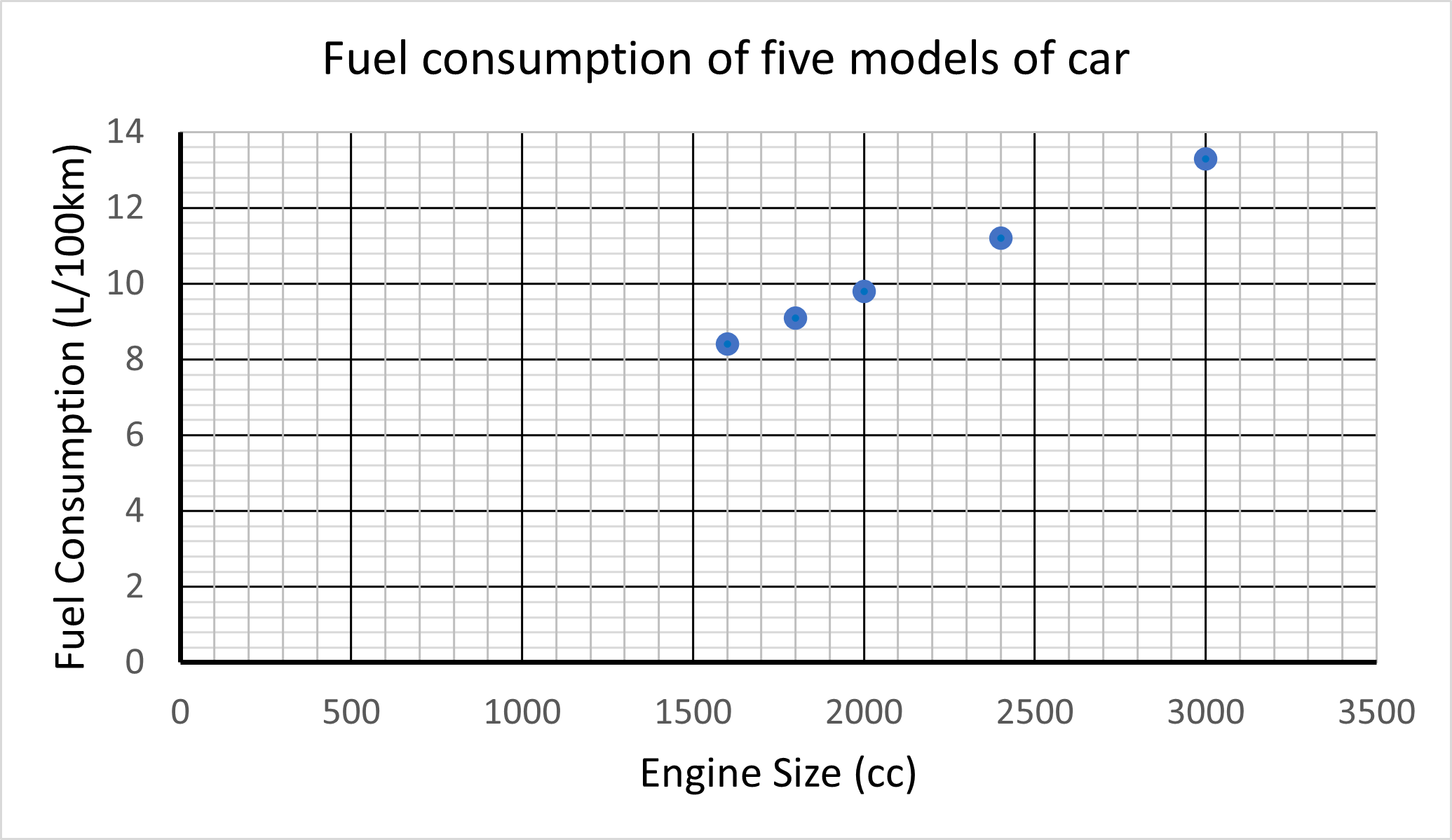   
    
   Discussion arising from activity: 
   • Which is the most efficient engine? How do you know? 
   • Why might someone choose to purchase the less efficient model? 
   • If the cars have a 40L fuel tank, how far can each car be driven between fills? How did you work the figures out? 
   • These data describe average fuel efficiency. What are some ways that the way a car is used will affect its efficiency? 
   • Note – these data appear to form a straight line. However, only a small range of engine sizes could be considered. Would it be realistic to have a point on this graph that related to, for example, 500 cc? 

3. Use the graph of fuel consumption (L/100km) for different engine sizes to create a table of data. Slide 3 of PowerPoint 2 has the table.   

   Engine size (cc)	Fuel consumption (L/100km)
   1600	8.4
   1800	9.1
   2000	9.8
   2400	11.2
   3000	13.3

4. Pose the question: What distance would each model be expected to travel on 10 litres of fuel?    
   Let students work in small teams to find answers. Roam, looking for: 
   • Do students understand the rate of litres per 100 kilometres? 
   • Do students work out a unit rate of kilometres per litre? 
   • Do students know how to find a multiplicative operator between amounts? 
   • Do they tend to work in kilometres per litre (between measures) of treat the measures separately (within measures)? 

5. Bring the class together to share ideas. Try to build on strategies students use, however inefficient they may be. Support students to represent the problem using effective recording, including ratio tables and equations.    
   Slides 4-6 scaffold thinking towards an answer for the 1600 cc model using a unit rate strategy.     
   Slide 7 uses a between strategy to find the unit rate for kilometres per litre. Answers are:  

   Engine size (cc)	Distance on 10 litres of fuel
   1600	119.05
   1800	109.9
   2000	102.04
   2400	89.29
   3000	75.19

6. Describe the overall trend of this relationship. 

7. Use the graph of distance travelled on 10 litres of fuel for different engine sizes (see slide 8 of PowerPoint 2).   

   Engine size (cc)	Fuel efficiency (km/L)
   2500	10
   2000	11.5
   1800	12.1
   2200	10.8

8. Provide students with Copymaster 1. Use slide 8 to show poor attempts to find a line of best fit.     
   How will we judge if the line of best fit is ‘the best fit’?    
   It should be straight, acknowledging that other models of relationships are sometimes useful (The actual line of best fit is a hyperbola).    
   It should minimise the distance between the points and the line. 
9. Invite students to draw in a line a best fit using Copymaster 1 and check using slide 8.     
   How would you describe the line? Use terms such as linear or non-linear, increasing, decreasing or constant.    
   What does the line tell you about the distance cars travel on 10 litres and engine size?    
   How far would you expect a 2200 cc model of the same type of car travel on 10 L of fuel? Slide 9 shows how to estimate the answer using the line of best fit.
10. Other problems:    
    High achieving students might try to write a formula for the line of best fit     
    (y = -0.0308x + 165.66) or alternatively use a spreadsheet or graphic calculator to find it.     
    Given that petrol costs an average of $2.53 per litre, what would you expect a 300 km trip in an 1800 cc car to cost in fuel?    
    How much more expensive would the same trip be in a 2200 cc car?     
    Would you expect this trend to apply for very small (e.g., 1000 cc) and very large (4500 cc) engines? Explain why the linear relationship may not hold.

Session 3

Focussing on using rates and proportions to compare data.

1. Use slide 1 of PowerPoint 3 to discuss the different nozzles found at a petrol bowser (pump). Some students will know that different nozzles provide different types of fuel. Petrol is available in 3 grade or octanes, 91, 95 and 98. The higher the number, the higher the capacity of the fuel to resist detonation therefore the more power it produces in the engine. You might look up a video online that discusses octane ratings. 
2. Introduce this problem using slide 2.     
   A test was carried using the same mid-sized car, using the three percentage concentrations of octane available in New Zealand petrol stations; 91, 95, 98. The car was first tuned to the fuel concentration, then with 15 L of that fuel in the tank, the car was driven until the tank was empty. This was repeated for each of the fuels.     
   The results were:    
   91-octane:  The car travelled 230 km on 15 litres of fuel.    
   95-octane:  The car travelled 237 km on 15 litres of fuel.    
   98-octane: The car travelled 242 km on 15 litres of fuel.    
   If the relationship between amount of fuel used and distance travelled is linear, how far would the car have travelled using:  
   • 7.5 litres of 91-octane petrol? 
   • 10 litres of 95-octane petrol? 
   • 6 litres of 98-octane petrol?
3. Discuss the problem to clarify what is required. Ask students to work in pairs with access to calculators.  Roam as students work. Look for the following: 
   • Is their recording supportive of making sense of the problem? (Look for use of ratio tables, number lines and equations) 
   • Do they approach the problem multiplicatively, by looking for common factors? 
   • Do they check that their answers are realistic, given the information? 
4. After a suitable time gather the class to process answers. Listen to students’ strategies first and after that use slides 3-6 of PowerPoint 3 to offer other ways to solve the problem that students may not have considered. Explain the representations where necessary.
5. Consider the test undertaken with the three octane rating fuels.   
   What conditions/variables were held as constant as possible when comparing these fuels?     
   Why would controlling those variables be important?   
   Revisit the data:    
   91-octane:  The car travelled 230 km on 15 litres of fuel.    
   95-octane:  The car travelled 237 km on 15 litres of fuel.    
   98-octane: The car travelled 242 km on 15 litres of fuel. 
6. Show students the graph on slide 7 of PowerPoint 3    
   What does this graph show?    
   Is the relationship linear? How do you know? (Animate the line y=1.75x+70.75 if needed)    
   Was this what you might have expected? Why/why not? 
7. Use slide 8 of PowerPoint 3:    
   On the day of the test this was the price of the three types of fuel:   
   91-Octane cost $2.45 per litre    
   95-Octane cost $2.65 per litre    
   98-Octane cost $2.77 per litre   
   Assume the car can be tuned to run on any of these three fuels.    
   What fuel gives the best value per 100 kilometres?
8. Ask students to investigate which fuel gives the best value. Look to see that they use representations to ease memory load and support their thinking. Answers are provided on slides 9-11.    
   What do the calculations show?    
   91-Octane is the cheapest per 100km. Obviously 98-Octane gives better engine performance but comes at a cost.

Session 4

Focusing on finding and describing a rate of change, for data given from a linear trend. 

1. A popular petrol fuelled car has an average petrol consumption of 7.6 L per 100 km travelled. A similar sized hybrid (electric and petrol) car uses an average of 3.9 L of petrol per 100 km without any further external charging.     
   How far would the petrol car travel on 3.9 L of petrol? 
2. Ask students to work in teams to solve the problem. Allow access to calculators. Roam as they work, looking for use of appropriate representations (see slide 2).    
   What calculation will give us the answer efficiently?    
   This diagram shows how the calculations can be found using within and between strategies. For example, (3.9/7.6)×100=51.32 km.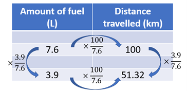    
    
   To make sense of the operators between numbers, students need to recognise that a fraction like 3.9/7.6 can be regarded as the dual operation “divide by 7.6 and multiply by 3.9” in any order. Those operations are those that would be carried out if 7.6 was transformed multiplicatively into 3.9.    
   Discussion arising from activity: 
   • How can the hybrid manage to make such a fuel saving without external charging? 
   • What are the advantages of petrol vehicles over hybrid?  
   • What are the advantages of hybrid vehicles over petrol?  
3. Set these problems for independent work (see slide 3 of PowerPoint 4):   
   A hybrid car has a petrol consumption of 3.9 L per 100km and uses 95-Octane at $2.65 per litre. A petrol car has a consumption of 7.6 L per 100km and uses 91-Octane at $2.45 per litre.  
   1. What is the cost of driving the hybrid car for 100 km? 
   2. What is the cost of driving the hybrid car per km? 
   3. What is the cost of driving the petrol car for 100 km? 
   4. What is the cost of driving the petrol car per km? 
   5. Find the percentage savings in the cost per km of fuelling the hybrid car over the petrol car. 
4. Answers are provided on slide 4. Question 5 is likely to prove the most difficult. It compares the cost per kilometre of running the hybrid compared to the petrol car. So the base is $0.19 per km or 19 cents/km. As a fraction the relationship of hybrid cost to petrol cost equals 10/19 = 0.5263 or 52.63%. Since 100 – 52.63 = 47.37 the saving is 47.37%. 
5. Pose this problem (slide 5). Ask students to work in teams.   
   A hybrid car has a petrol consumption of 3.9 L per 100km and uses 95-Octane at $2.65 per litre. A petrol car has a consumption of 7.6 L per 100km and uses 91-Octane at $2.45 per litre. The average driving distance of a single car is 14 000 per km per year. 
   1. What is the cost of driving the hybrid car for 14 000 km? 
   2. What is the cost of driving the petrol car for 14 000 km? 
   3. Calculate the expected average fuel savings for running the hybrid over the petrol car in this example. 
6. Roam as students work. Look for the following: 
   • Do they use efficient calculations to solve each part? 
   • Do they fall back to more helpful representations, like ratio tables, if they get stuck? 
   • Do they check their answers for reasonableness? 
7. After a suitable time bring the class together to discuss strategies and answers. 
8. Use slide 6 to provoke discussion about efficient strategies. Ask students to compare their strategies with those shown. 
9. Use slide 7 to pose this problem for students to work on in small teams:   
   Tom has a petrol car but wants to change if for a hybrid. Use the following information to estimate the time it would take for Tom to recover the cost of upgrading from his petrol car to a hybrid.  
   1. A hybrid car has a petrol consumption of 3.9 L per 100km and uses 95 octane at $2.65 per litre. A petrol car has a consumption of 7.6 L per 100km and uses 91 octane at $1.45 per litre.  
   2. The average driving distance of a car is 14 000 per km per year. 
   3. To trade his petrol car in for a hybrid, it will cost Tom $7 500.  

Session 5

Focusing on finding, describing, and applying a linear relationship. 

1. Pose this problem (slide 1 of PowerPoint 5):   
   Before changing to a hybrid or electric vehicle Mere checks out the depreciation of these three types of cars. Depreciation is the loss in sale price as the car ages.   
   She uses these average sale figures from the car dealers’ Red Book for 3 comparable models.   

   Model	2020 (New)	2021	2022	2023	2024
   Petrol	32,000.00	24,000.00	18,000.00	13,500.00	10,130.00
   Hybrid	48,900.00	42,500.00	36,100.00	29,500.00	16,700.00
   Electric	64,000.00	62,500.00	61,000.00	59,500.00	58,000.00

2. To look for patterns, Mere graphs the data (See slide 2 of PowerPoint 5).    
   Ask students to discuss these questions in small groups.
   • What patterns can you see?   
     Students might notice that the electric car is expensive to buy but holds its value well. Both the petrol and hybrid cars decrease in value quickly. However, the hybrid has a sudden drop in value from the 3rd to 4th year. That might be due to the prospect of replacing the battery. The loss of value in the petrol model seems to be flattening off after 3 or 4 years.
   • What might the value of each model be in 2025?   
     Students might expect the electric to lose little value based on the previous 4 years. The pattern is for the car to lose $1,500 per year in value. They might expect the value of the hybrid to drop a lot again, or alternatively think the loss in value will be much less in 2024-2025. If the petrol car continues to depreciate by a factor of about 0.75 it should be valued at 0.75 x 10,130 = $7,601 in 2025.
3. Gather the class to discuss answers. Expect students to justify their conjectures about future values and explain why they think the cars have different patterns of depreciation.   
   Which model has a depreciation pattern that is almost linear? (Electric)   
   How would you describe the depreciation pattern for the petrol model?   
   Students may not know the exponential decay model, so you may need to explain it. Use other examples, such as the cooling of hot liquid over time, amount of drug in a patient’s body over time, or radioactive decay (used in carbon dating).
4. Extend the linear pattern of depreciation for the electric car by posing the following:    
   Use the table of graph to predict the value of the electric car in 2040.    
   Is the prediction realistic? Explain why.   
   Let students use Copymaster 2 to work out their predictions. Students might extend the table using the constant first order difference between terms of $1,500 per year and transfer the ordered pairs to the graph. After 20 years the electric car has a predicted value of $34,000. Ask students if they think that is a realistic prediction. 
5. Use slide 4 of PowerPoint 5 to introduce this problem:   
   Mere expects to travel about 15 000 km per year, whatever car she gets. That includes her daily commute to work which is a big cost to her. Usually, she keeps her cars for 5 years before trading in and buying a replacement.    
   Mere wonders if changing her petrol car to a hybrid or an electric car is worth it.    
   What information will Mere need to make an informed decision? 
6. Let students work in small teams to decide what information they will need. The problem is complex so expect a wide range of suggestions. These might include: 
   • Value of her current car. 
   • Initial cost of a new vehicle. 
   • Value of the car that is likely after 5 years, factoring in depreciation. 
   • Running cost per year for each type of vehicle that includes servicing, insurance, and registration. 
   • Payments for a car loan. 
7. Students might look up these costs. However, for efficiency use the cards from Copymaster 3 to provide students with the information they need. Students might sort the cards by vehicle type to make calculation easier.    
   What order will you do you calculations for each model of car?    
   How will you organise your calculations? 
8. Let students model the problem in small team, offering scaffolding where needed. A model spreadsheet is included as slide 5 but refer to it only if needed. The net position favours the electric car but that is dependent on Mere’s ability to service the loan that costs almost $14,000 per year. The loan cost for the petrol car is about $4,500 per year which is more affordable.

Session 6

Using a linear model to solve problems. 

1. Pose this problem about speed, using slide 1 of PowerPoint 6.    
   Audrey commutes to work on her scooter.    
   The one-way trip is 12 kilometres.    
   She averages a speed of 40 kilometres per hour which includes the stops she makes.     
   How long is each trip to work, in minutes?
2. Let the students attempt the problem. Roam as they work. Look for: 
   • Do they see that 40 km/hr is a rate? (A rate is relationship between two measures, distance and time in the case of speed) 
   • Do they connect the previous problems about fuel consumption and cost to this context about speed? 
   • Do they apply the representations learnt in previous sessions to this problem? 
   • Do they convert the rate of 40 km/hr to a rate per minute?
3. Gather the class to share strategies and answers (slide 2 can be used if needed). Use examples from the students to highlight useful ways to represent the problem.    
   For example, a ratio table is a good way to record the calculation steps.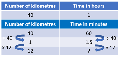    
    
   Likewise, a double number line supports strategies: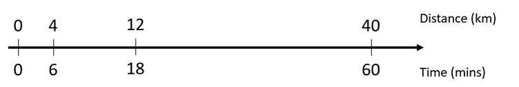    
    
   Where students carry out calculations, ask them to explain what the numbers in the calculation refer to. For example:    
   “I divided 60 by 40. That gave me 1.5 which is the number of minutes Audrey takes to travel 1 kilometre.”    
   “I divided both 40 and 60 by 10. That showed me that Audrey travels 4 kilometres in 6 minutes.” 
4. Provide similar speed related problems for students to work on (see slides 3-16 of PowerPoint 6). Look for students to identify similar characteristics in the problems, such as a rate in km/hr and a time or distance given.
   1. (Slide 3) Kadijah walks to work each day.    
      The fitness app on his watch shows that he walks at a speed of 6.4 kilometres per hour.    
      If the distance from Kadijah’s home to work is 4.8 kilometres, how much time does he take to walk it?    
      Solution strategies are presented on slide 4. 
   2. (Slide 5) Luciana catches the bus to work each day.    
      On her Public Transport app the road distance of her trip shows as 7.2 kilometres.    
      The bus averages a speed of 24 kilometres per hour over that distance.    
      How long, in minutes, is the Luciana’s bus trip?   
      Solution strategies are presented on slide 6. 
5. Sometimes in a speed-related problem the time is unknown. Other problems present the distance as unknown. Let students work in small groups. Use PowerPoint 6 to pose these problems, though slides 9-12:
   1. Keola and Lupelele complete 2 circuits of Rata Park on e-scooters.    
      They ride for 13 minutes and 12 seconds at a speed of 10 kilometres per hour.    
      What distance, in kilometres, is equal to 2 circuits? 
   2. Alec catches the train to work.    
      The journey takes 75 minutes at an average speed of 88 kilometres per hour.    
      What distance, in kilometres, is Alec’s train journey?
6. Progress to problems in which the speed is unknown. Let students work in small groups. Use PowerPoint 6 to pose these problems, through slides 13-16:
   1. Rosalie drives to her polytechnic to study.    
      The drive is 24 kilometres and takes her 18 minutes.    
      What is Rosalie’s average speed, in kilometres per hour? 
   2. Lorenzo jogs 8.4 kilometres every lunchtime.    
      The run takes him 40 minutes.    
      What is Lorenzo’s average speed, in kilometres per hour?
7. Present situations involving constant speed graphically. Slides 17 and 18 present the Rosalie and Lorenzo situations graphically. In each case explore how the time taken to travel different distances can be found, as points on the graph, if speed is constant.