Randomisation

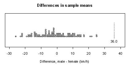
The use of methods involving elements of chance, such as random numbers, to allocate individual units to groups.

Randomisation used in data collection

Randomisation is used in experiments by using methods involving elements of chance to allocate individual units to treatment groups. Further detail is provided in the paragraph on randomisation in the description of experimental design principles.

Randomisation forms the basis of many sampling methods, including random sampling, simple random sampling, cluster sampling and stratified sampling.

Randomisation used in statistical inference

Randomisation is used at Level Eight in a resampling method for making statistical inferences from data. This method is illustrated in the following two examples that compare two means. A summary of the method is provided after these two examples.

Example 1

An assertion is made that male University of Auckland students tend to reach faster driving speeds than female students. To investigate this, random samples of 20 male and 20 female University of Auckland students were asked how fast they had driven, to the nearest 10km/h.

The values obtained were:
Males:    130 120 120 140 140 120 120 120 170 160 110 150 210 240 200 140 150 200 240 140
Females:    100 170 140 120 120 120 120  90 120 100 130 120 120 130 120 120 110 100 130 120

The sample means are = 156.0 km/h for the males and = 120.0 km/h for the females. From this data, an estimate of the difference between the population mean fastest speeds for males and females is - = 36.0 km/h.

A dot plot of the data is shown below.

Does the data provide any evidence to support the assertion? In other words, could a difference as big as the observed difference of 36.0 be produced just by chance?

If the numbers are considered as just showing the natural variability in fastest driving speeds among such university students, then would random allocation of the speeds from these two samples to the male and female groups often produce a difference in sample means as big as 36.0? If random allocation alone could easily produce a difference as big as 36.0 then the data cannot be interpreted as support that the mean fastest driving speed for males is greater than the mean for females.

The speeds from the two samples are combined and 20 of them are randomly allocated as speeds for the males, leaving the other 20 as speeds for the females. This is equivalent to assuming there is no link between fastest driving speed and gender. The difference in the sample means is an estimate produced by sampling variation alone. One such randomisation is shown below.

The sample means are = 139.0 km/h and = 136.5 km/h, with - = 3.0 km/h.

Another random allocation of 20 (of the 40) as speeds for the males, leaving the other 20 as speeds for the females is shown below.

   
The sample means are = 132.5 km/h and = 143.5 km/h, with - = -11.0 km/h.

Continuing this process for a total of 100 such random allocations produced differences in sample means shown in the dot plot below.

Of the 100 differences produced by sampling variation alone, none was as large as the observed difference of 36.0 km/h produced by the two samples. This shows that a difference of 36.0 km/h or larger is very unlikely to be produced by sampling variation alone when there is no link between fastest driving speed and gender. It can be concluded that the data provide very strong evidence that the mean fastest driving speed for male University of Auckland students is greater than that for females.

Note that the assertion was that the mean fastest driving speed for males is greater than that for females and so only positive differences of 36.0 or more were considered when forming the conclusion.

Example 2

Question: Is there a difference in the average daily number of text messages sent by male and female University of Auckland students? To investigate this, random samples of 20 male and 20 female University of Auckland students were asked how many text messages they typically sent in a day.

The values obtained were:
Males:     40  10  30  20   5   0   1  30  30  10  30   3   6  50  20 30  20  50  10  30
Females:     20   2  50  30  15   0   6  60  10   5 100  15  40   3  30 15 100   5   5  50

The sample means are = 21.25 messages per day for the males and = 28.05 messages per day for the females. From this data, an estimate of the difference between the population mean daily number of text messages for males and females is - = -6.80 = messages per day.
 
A dot plot of the data is shown below.

Does the data provide any evidence of a difference in the average daily number of text messages sent by male and female students? In other words, could a difference as big as the observed difference of –6.80 be produced just by chance?

If the numbers are considered as just showing the natural variability in daily numbers of text messages sent among such university students, then would random allocation of the number of messages from these two samples to the male and female groups often produce a difference as big as –6.80? If random allocation alone could easily produce a difference in sample means as big as
–6.80 then the data cannot be interpreted as support that the mean daily number of text messages sent is different for males and females.

The numbers of messages from the two samples are combined and 20 of them are randomly allocated as daily numbers of text messages sent for the males, leaving the other 20 as daily numbers of text messages sent for the females. This is equivalent to assuming there is no link between daily number of text messages sent and gender. The difference in the sample means is an estimate produced by sampling variation alone. One such randomisation is shown below.

 The sample means are = 31.45 and = 17.85, with - = 13.60.

Another random allocation of 20 (of the 40) as daily numbers of text messages sent for the males, leaving the other 20 as daily numbers of text messages sent for the females is shown below.

The sample means are = 33.80 and = 15.50, with - = 18.30.

Continuing this process for a total of 100 such random allocations produced differences in sample means shown in the dot plot below.

Of the 100 differences produced by sampling variation alone, 52 (52%) were at least as far from zero as the difference of –6.80 produced by the two samples. This shows that a difference of –6.80 is a typical value produced by sampling variation alone when there is no link between daily number of text messages sent and gender. It can be concluded that the data provide no evidence that the mean daily number of text messages sent by male University of Auckland students is different from that for female students.

Note that the question was about a difference between the means for males and females and so positive and negative differences that are at least 6.80 from zero were considered when forming the conclusion.

Note: The principles explained in the above examples can also be applied to a difference between two proportions for category variables and to a slope of a fitted regression line for bivariate measurement variables.

Summary

Data are collected to investigate an assertion or a question, usually involving a comparison of a numerical variable between two categories of a category variable (i.e., that there is a link between the numerical variable and the category variable). An estimate of a population parameter is calculated from the data. This observed estimate is often a difference between means (as in the two examples) but could be a difference between two proportions or a slope of a fitted regression line.

Could an estimate as big as the observed estimate be produced just by chance?

To answer this question, the effect of sampling variation alone on the estimate needs to be considered when it is assumed that there is no link between the two variables. If random allocation alone could easily produce an estimate as big as the observed estimate then the data cannot be interpreted as support for the existence of a link between the two variables. Values of the numerical variable obtained from the data collection are randomly allocated to the two categories of the category variable. An estimate is calculated from this ‘resampling using randomisation’ process. This process is repeated many times to form a distribution of estimates under sampling variation alone.

By comparing the observed estimate with the distribution of estimates, an assessment can be made of the strength of evidence the data provide for the assertion or provide for a conclusion to the question. This assessment is made by looking at the percentage of estimates under sampling variation alone that are at least as far from zero as the observed estimate.
 
Why are estimates that are at least as far from zero as the observed estimate considered?

If the observed estimate is a typical value of an estimate produced by sampling variation alone then it is quite believable there is no link between the variables. In this case, a relatively large percentage of estimates produced by sampling variation alone will be at least as far from zero as the observed estimate.

If the observed estimate is not a typical value of an estimate produced by sampling variation alone then it is difficult to believe there is no link between the variables. In this case, a relatively small percentage of estimates produced by sampling variation alone will be at least as far from zero as the observed estimate.

This makes the percentage of estimates produced by sampling variation alone that are at least as far from zero as the observed estimate an appropriate measure of the strength of evidence that there is a link between the two variables, with smaller percentages providing stronger evidence of a link.

Estimates produced by sampling variation alone are usually values of a continuous random variable (but the values are rounded). Because of the continuous nature of the values of these estimates, the percentage of estimates that are the same distance from zero as the observed estimate will almost always be small, causing this to be an inappropriate measure of the strength of evidence of a link.

See: resampling, strength of evidence

Curriculum achievement objectives references
Statistical investigation: Levels (5), (6), (7), 8