This unit teaches students to identify linear relationships and solve linear equations in context.
- Identify and find values for variables in context.
- Identify linear relationships in context, including those with negative rates of change.
- Represent linear relationships using tables, graphs and simple linear equations.
- Draw strip diagrams to represent linear equations, including those with negative co-efficients of the independent variable.
- Solve linear equations and interpret the answers in context.
Algebra started with the need to solve problems. Al Khwarizmi, a Persian mathematician, was arguably the first person to represent linear and quadratic problems in symbolic form and solved the problems by processes of ‘restoration’, i.e. equivalent operations that conserved equality. In fact, the word for algebra comes from the Arabic word for restoration.
It is fitting then that modern approaches to algebra focus on the thinking that underpins the symbolic systems. Algebraic thinking is concerned with generalisation. Letters, words, tables, graphs, networks, etc. are cultural tools that enable us to represent, then think with, those generalisations. With representational tools we are capable of ‘amplified cognition’ in that we can anticipate results that would never be possible if we relied solely on the physical environment, and on our limited capacity to process ideas just mentally.
Generalisation begins with noticing patterns and structures. A pattern is a consistency, that is something that occurs in a predictable way. It is the ‘what’ of algebraic thinking. Structure is about the organisation of patterns. It is the ‘how’ and sometimes the ‘why’ of generalisation. From noticing pattern and structure, we develop properties. For example, early counting involves pattern and structure. The ‘fourness’ of a collection comes from noticing sameness among collections of four, irrespective of the size, colour, texture, etc. of the objects. Structure of counting involves ideas like the order of counting the objects doesn’t matter.
Specific Teaching Points
In upper primary school, learning experiences for algebraic thinking typically begin with patterns. Usually these patterns are spatial and may be connected to some meaningful life context, though number patterns are also rich in opportunity. Patterns involve variables, that is features, some of which can be quantified. For example, consider this simple spatial pattern.
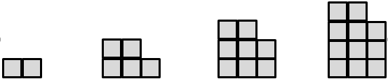
Among the variables we might discern that the ‘tower’ has height and each ‘tower’ is made of some number of squares. Height and number of cubes may not be the only variables, just those we notice. Variables change, that is height varies and so does the number of squares in the ‘tower’. We might try to find a relation between the variables, describe and represent that relation, and use it to predict how the pattern grows beyond what we can see. Then we are thinking with the properties and representations in a sophisticated way.
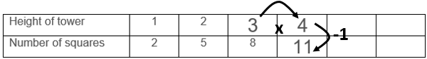
On the way it is likely we will need to organise the data from the pattern systematically. A table of values is a productive generic strategy, so we represent the pattern like this:

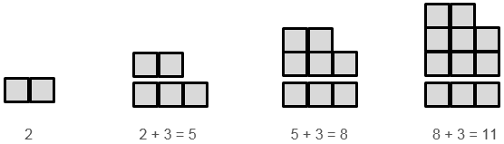
The danger in moving to an organised numeric strategy like a table too early is that it may negate what we can ‘see’ in the pattern visually. Noticing and reasoning may be inductive, that is tied to the incremental change of the figures. For example:
Noticing and reasoning can also be abductive, that is based on the structure of one example.
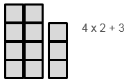
Noticing and reasoning can be deductive, that is based on making assumptions about structure and reasoning with the assumptions. For example, we might assume that the tower is composed of an array of something multiplied by three plus two.
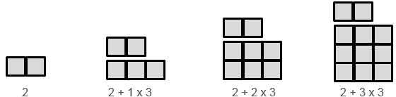
From the assumptions made, we might deduce the appearance of towers much further on in the sequence, e.g. A tower 100 high will contain 2 + 99 x 3 squares. Ways of ‘seeing’ the pattern are manifest in relations within the table of values. For example, inductive thinking leads to seeing the values in the bottom row increasing by three each time. Abductive reasoning might support seeing this relation in the table:
Representing the relation as an algebraic equation involves two important and connected types of knowledge, related to the language conventions (semiotics), and to the nature of variables. We might write s = 3h – 1, or s = 3(h - 1) + 2, or s = 2h + (h – 1), depending on what we notice. The equations are meaningless to anyone else unless we clearly define what the variables, s and h, represent. Note that both and s refer to quantities that vary and are not fixed objects, such as houses or towers. Quantities are a combination of count and measurement unit. In this case h expresses unit lengths in height, and s refers to an area of squares. 3h means h multiplied by three, not thirty-something, and 3(h - 1) means that one is subtracted from h before the multiplication by three occurs.
Working with variables requires acceptance of lack of closure, that is thinking with an object (h in this case) without specifically knowing what it is. For example, knowing that 3(h – 1) = 3h – 3 is true, irrespective of whatever the value of h, is itself a generalisation. The equals sign represents a statement of ‘transitive balance’ meaning that the balance is conserved if equivalent operations are performed on both sides of the equation. Knowledge of which operations conserve equality and those which disrupt it are important generalisations about the properties of numbers under those operations, e.g. distributive property of multiplication.
This unit specifically deals with linear relations. The first sign of linearity is that there is constant difference in the increase or decrease of one variable, as the value of the other increases by one. In the table above the number of squares increases by three as height increases by one.
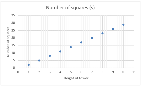
Note that this graph shows a relation, not a function, since the values of variables are discrete, not continuous. There are some important connections between features of the algebraic equation, the table, and the graph of a linear relation. Constant difference is represented by the co-efficient of the independent variable (s = 3h -1 in this case), differences of three in the bottom values of the table, and a slope of three (change in s for every unit change in h). The constant in the equation (- 1) is reflected in the table by a need to adjust the value of 3h by subtracting one to get the value of s, and reflected in the graph as a downward translation (shift) of the graph for s = 3h by one unit. This results in the intercept of the graph with the s axis being (0, -1), not the origin (0, 0).
Simple linear equations occur when the value of one variable in a relation or function is set and the other must be found. For example, with the tower problem this problem might be posed; “A tower in the pattern has 98 squares. How high is the tower?” Depending on the equation used to represent the relation, this problem can be expressed as 3h – 1 = 98, 3(h – 1) + 2 = 98 or 2h + (h – 1) = 98. Linear equations with the variable on both sides occur when two conditions are equalised. An example might be, “Both Lilly and Todd look at the same tower. Lilly notices that the number of squares in the tower is three times the height less one. Todd notices that the number of squares is two times the height plus 18. How tall is the tower?” This problem can be written as 3h – 1 = 2h + 18.
The learning opportunities in this unit can be differentiated by providing or removing support to students and by varying the task requirements. Ways to support students include:
- modelling the construction of strip graphs, tables, and the use of equations
- grouping students flexibly to encourage peer learning, scaffolding, extension, and the sharing and questioning of ideas
- providing opportunities for students to create their own problems that apply the mathematics introduced in this unit within a relevant, meaningful context
- applying gradual release of responsibility to scaffold students towards working independently
- roaming and providing support in response to students' demonstrated needs
- providing frequent opportunities for students to share their thinking and strategies, ask questions, collaborate, and clarify in a range of whole-class, small-group, peer-peer, and teacher-student settings.
Te reo Māori kupu such as kauwhata tāhei (strip graph), taurangi whakamauru (dependent variable), taurangi wehe kē (independent variable), whārite rārangi (linear equation), and pānga rārangi (linear relationship) could be introduced in this unit and used throughout other mathematical learning.
- Attachments as listed at the bottom of the unit
- Access to the two digital learning objects:
- Interactive whiteboard, data projector, a smart TV, or similar (to allow students to see videos and PowerPoints on a large screen)
- Access to Excel or a similar spreadsheet program
Prior Experience
It is anticipated that students at Level 4 and 5 understand, and are proficient with, multiplicative thinking. However, the tasks in this unit are also accessible for students whose preference is additive thinking. In fact, the experiences may prompt a move towards multiplicative thinking.
Session One: Danny’s Ice cream Truck
Use the Session One video to structure this session. The video commentary prompts you to stop at certain points to allow students to discuss the ideas in pairs or threes. In this session students investigate the context of an icecream seller. The relation between time (t), in minutes, and units left in the reservoir (u), is linear but involves a negative co-efficient. Students are encouraged to connect strip diagrams, graphs and equations as problem solving tools.
The first minute introduces Danny, the icecream seller. A graph is then presented with only three points showing. Students need to make sense of each point as representing a pair of values for the independent variable, time in minutes (t), and the dependent variable, units remaining (u). So, the point (18, 146) refers to Danny observing that 18 minutes after opening there are 146 units remaining in the reservoir.
The next section of the video focuses on the relation between time (t) and the number of units (u) being linear. What can students ascertain about the relation? Rate of change is particularly significant in this context. How many units is Danny using up each minute? That rate is represented by the slope of the line, sometimes described as ‘rise over run’. Consider this enlarged picture of the change between (12, 164) and (18, 146).
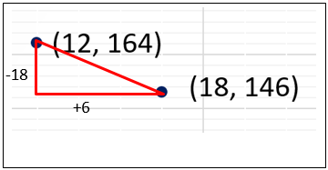
So, as time (t) increases by six minutes the number of units (u) decreases by 18. The rate of decrease is -3 units per minute (dividing both -18 and 6 by 3 to get a unit rate). Students may describe how the amount used up could be represented as 3t, the number of minutes multiplied by three.
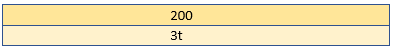
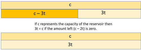
A strip diagram of the situation is introduced. The strip showing 200 represents the total capacity of the reservoir. 3t represents the rate of change, 3 units consumed for every minute, and 200 – 3t represents u, the number of units remaining in the reservoir. Students should note that 200 remains constant and 3t and 200-3t (u) co-vary. As 3t increases 200 – 3t (u) reduces.
The remainder of the video poses the problem of when the reservoir is empty, i.e. 200 – 3t = 0. Students may make the inference that for 200 – 3t to equal zero, 3m = 0. The progression in strip diagrams leads to this representation as 200 – 3t gets smaller.
As an equation the solution is:
200 – 3t = 0
200 = 3t (adding 3t to both sides)
66⅔ = t (dividing both sides by three)
The strip diagram makes the division by three obvious. A value for t = 66⅔ when u = 0 matches a prediction from the graph of where the line will intersect the horizontal axis.
Provide the students with Copymaster One which contains variations of the Danny problem. Encourage the students to work in small groups to solve the problems. The problems explore what happens to the time at which u = 0 for different rates. It also explores how Danny can change the reservoir for one with greater capacity.
As the students work, look for:
- Do the students identify rates of change from points on the graph?
- Do they adjust the formula for finding when the reservoir will be empty?
- (for example, if the rate is 4 units per minute they solve 4m = 200, so t = 50)
- Do they apply sensible approximation methods to find the capacity of a reservoir that lasts 2 hours?
- Do they use the fill down function of the spreadsheet effectively?
Bring the students together as a class to discuss the teaching points above. Video Two models how the final problem can be solved using a spreadsheet. Trial and improvement can be a time-consuming strategy so encourage the students to also try equation based techniques. That might involve drawing a strip diagram like this:
If t has to be 120 then the equation is simply u = 3t, so u = 3 x 120 (substituting t = 120).
Session Two
This session provides another context for modelling with linear equations where the co-efficient of the independent variable is negative. The Session Two video can be used to run the session with places for pausing to allow for student discussion. The scenario is that of a gang demolishing a building, the variables being time in number of days and sections of the building that remain.
The values given to the students are for days two, four and seven. So the ordered pairs are not consecutive and the initial number of sections in the building needs to be found. The crew removes six sections per day so the rate is constant and negative. The relation is linear because plotting the given ordered pairs will show points that exist on a line.
Problems are posed for the students to solve and the rate is confirmed to be constant and negative. Allow the students time to solve the problem (Question Two) in small groups before gathering the class. Permit access to spreadsheets as a useful tool. This problem could be represented by the equation 144 – 6d = 40, with d representing the number of days and s assuming a fixed value of 40.
Look for the following:
- Do the students recognise that the rate is negative six? (a reduction of six in sections for an increase of one in the number of days)
- Do they use that rate to work backwards to establish the building contained 144 sections on Day Zero?
- Do they use inductive or deductive rules to work out the answer?
An inductive rule involves recursively taking away six until 40 sections remain. Then the number of counts of minus six are tracked to establish the value of d for which s = 40.
A deductive rule would be multiplicative in nature. For example, 144 – 40 gives the number of sections to be removed. 104 ÷ 6 = 17 r4 gives the number of days (round to 18) required.
Do any students use an algebraic equation to solve the problem?
After a suitable period gather the class to discuss their methods. Session Two video A provides a discussion of how a spreadsheet might be used to solve the problem. Session Two video B introduces the idea of using algebraic methods to solve the equation. Encourage students draw a strip diagram for the demolition problem first before showing the video. The diagram can be represented by several different equations all of which are legitimate forms.
The situation is authentically represented by:
144 – 6t = 40
144 = 40 + 6t (adding 6t to both sides)
104 = 6t (subtracting 40 from both sides)
17⅔= t (dividing both sides by six)
Copymaster Two provides students an opportunity to explore variations of the demolition problem. Encourage students to work collaboratively on the problems before bringing the class together to discuss their solutions.
Session Three
The session is devoted to using the third and fourth learning objects in a collection about solving linear equations. The Algebra Learning Object 3 and Algebra Learning Object 4 videos introduce how to use the learning objects. The objects are accessible through these links:
Solving linear algebra equations (variable on one side, positive and negative values)
Solving linear algebra equations (variable on both sides, positive and negative values)
After some time devoted to using the learning objects gather the students together. Ask them how what they have learned could be useful in solving problems like Danny’s reservoir problem and Tanya’s demolition problem.
Session Four
In this session students investigate linear equations where the variable is present on both sides. The Session Four video presents a scenario of two siblings paying back money loaned to them by Grandparents. The dependent variable is the debt owing in dollars and the independent variable is time in weeks. Play the video, pausing at appropriate points to discuss matters that need clarification.
Make sure that the video is paused as students attempt to solve the problems. Look for the following:
Do students realise that the relation between weeks and debt is linear?
Can they form equations for the debts of Jakob and Saskia? In doing so do they define the variables clearly, recognise the negative rate as the co-efficient of w, and build the initial amount of the loan as a constant?
Do they apply the skills they have learned to use spreadsheets and equations to solve the problem?
After a suitable period bring the class together for students to share their strategies. Choose groups, or individuals, to highlight different ways to solve the problems. Given the focus on solving linear equations in Session Three expect that some students have used this strategy.
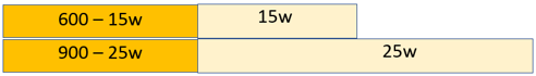
The variables, time in number of weeks (t or w) and debt in number of dollars (d) should be clearly defined. Suitable equations would be:
d = 600 – 15w or d = -15w + 600 (For Saskia) d = 900 – 25w or d = -25w + 900 (for Jakob)
Problem one involves setting the debt (d) at zero and solving for w.
0 = 600 – 15w (Saskia) 0 = 900 – 25w (Jakob)
So 15w = 600 So 25w = 900
So w = 40 So w = 36
Problem Two involves equating the two expressions for debt as:
600 – 15w = 900 – 25w and solving for w.
This equality might be represented as a strip diagram as used in the learning objects.
Solving for w by trial and improvement is very cumbersome so using algebraic methods is more efficient:
600 – 15w = 900 – 25w
So, 10w = 300
So, w = 30
Can the student interpret this answer in context? This mean in week 30 both Jakob and Saskia will owe the same debt.
What is that debt? (600 – 15 x 30 = 150 and 900 – 25 x 30 = 150).
How much will they save on their loans? ($150 each)
The Session Four A video shows how a spreadsheet might be used to solve both problems. If students rely entirely on spreadsheets encourage them to verify the results with other methods to build up their flexibility of strategies. Note that the graphs of the two debt functions intersect at (30, 150) which is the solution to problem two.
After the class have discussed possible solution strategies provide the students with Copymaster Four. This worksheet provides three problems to which the student can apply the algebraic techniques they have learned.
Two of the scenarios are familiar, demolition and icecream machine reservoirs. The solutions are as follows:
Problem One
Let d represent the number of days and s represent the number of building sections remaining.
- Crew A’s equation is s = 112 – 3d and Crew B’s equation is s = 148 – 4d
Set each equation for s = 0 gives solutions of d = 112 ÷ 3 and d = 148 ÷ 4.
- Equating the expressions gives 112 – 3d = 148 – 4d so d = 36
Problem Two
Let m represent the number of minutes and u represent the number of units remaining in the reservoir.
- Mr Blue u = 240 – 4m and Ms yellow u = 348 – 6m
Let u = 0 gives m = 60 and m = 58
- Equating the expressions gives 240 – 4m = 348 – 6m which has a solution for m = 54
Problem Three
Let b represent the number of boxes sold and bought.
The equation is: 50 + 12b = 458 – 12 b which has a solution at b = 17.
Dear Parents and Caregivers,
This week we are learning about linear relationships. Real life is full of situations where things grow or decline at a constant rate, such as the money we earn for the hours we work, or the total cost related to the quantity we buy.
We have been learning to represent linear relationships using tables of values, graphs and equations, and to use spreadsheets to solve problems with linear relations. Ask your child to share their learning with you.