In this unit procedural fluency and conceptual understanding are developed together. Students will represent quadratic relationships, particularly using graphs and equations, and will use quadratic functions to model phenomena such as paths of projectiles, stopping distances and profits. In turn, they will illustrate how mathematical modelling is used to make informed decisions in the real world.
- Make a table of one variable against another to represent a quadratic relationship.
- Represent a quadratic relationship between two variables in words and as an equation.
- Represent a quadratic relationship as a parabola on the Cartesian Plane.
- Recognise the key features of a parabola, including the vertex and x-intercepts.
- Use graphing software to ‘curve fit’ a quadratic model onto a set of ordered pairs.
- Apply quadratic functions to predict unknown values.
The parabola is one of the conic sections which are created by slicing two opposed cones with straight cuts. Ellipses, including circles as a special case, and hyperbolas are other well-known conic sections. The integration of algebra, in the form of quadratic equations, and the conics was made possible by Rene Descarte’s creation of Cartesian co-ordinates in the first half of the 17th century. Quadratic functions have a general form of y = ax2 + bx + c, where a, b and c are constants, and x and y are variables.
The concept of a variable can be difficult for students to grasp. A variable is a quantity that can take up different values. In algebra variables are represented as letters. We often refer to a letter symbol as a variable, where we sometimes mean an unknown specific value, a generalised unknown (lots of possible values), or a variable that changes in relation to other variables in a certain situation.
Before beginning this unit, students should be familiar with the construction of linear graphs with integer values and with the solving of simple linear equations. They should also have attempted the other two units on quadratics for Level Five (Mary's Garden and Array for Quadratics). Graphs provide an accessible visual representation of the relationship between two variables. Connecting graphs and equations from the same context supports students to understand how multiple representations connect and are useful for solving problems.
For a structured situation, research indicates that finding a rule for the general term can be a difficult for many students. Students often initially notice the iterative (recursive) rule that gives the value of a term of a sequence from the previous term. However, they are sometimes unable to find the general relationship between the independent and dependent variables, or apply the inverse relationship.
This unit should follow delivery of linear algebra and linear graphing, quadratic equations and graphing, at Level 5. The teaching of skills occurs within contexts that provide opportunities for discussion and development of procedures and concepts. As each learning outcome is explored there may be a need for consolidation through more traditional exercises, such as those found in text books, worksheets or online practice activities. Students who are quick to grasp these concepts will benefit from extension tasks such as those found in the Rich Learning Activities.
The learning opportunities in this unit can be differentiated by providing or removing support to students and by varying the task requirements. Ways to support students include:
- modelling the construction of tables, and graphing of functions
- providing pre-prepared tables and graphing templates for students to fill out
- grouping students flexibly to encourage peer learning, scaffolding, extension, and the sharing and questioning of ideas
- applying gradual release of responsibility to scaffold students towards working independently
- roaming and providing support in response to students' demonstrated needs
- starting and ending each session with a review of key knowledge
- providing frequent opportunities for students to share their thinking and strategies, ask questions, collaborate, and clarify in a range of whole-class, small-group, peer-peer, and teacher-student settings.
The context for this unit can be adapted to suit the interests and experiences of your students. Select examples of curves (parabolas) to ask your students to investigate, that are relevant to them and their learning (e.g. the trajectory of a netball, features of local buildings and artworks, rollercoasters). Perhaps you could generate a list of these contexts with your class.
Te reo Māori kupu such as whārite pūrua (quadratic equation), unahi (parabola), and akitu (vertex) could be introduced in this unit and used throughout other mathematical learning.
This unit of work is built around the vertex form of a quadratic equation, y = a(x-p)2+q. Students learn the effect on the corresponding parabolic graph of changing the variables, a, p and q. This understanding combined with the power of digital graphing packages allows them to create models for different phenomena.
The tool of curve fitting are introduced in the first three lessons then applied to two complex modelling situations, predicting braking distances of vehicles in variable situations and maximising profits for a business.
Session One: Finding simple quadratic functions using differences
In this session students connect the general form of simple quadratic functions with second order differences and graphs. Begin by showing Animations 1A, 1B and 1C. Students will need square paper or record in their exercise books.
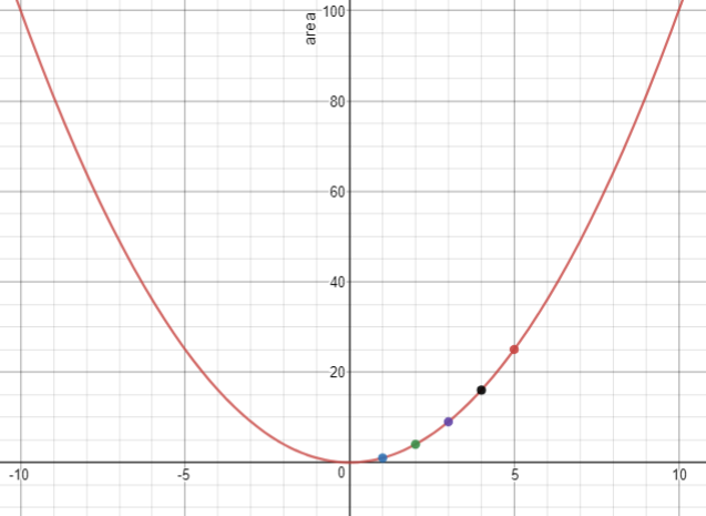
Animation 1A explores the function y = x 2 though enlarging the unit square by integral scalers. Look for students to:
- Recognise that a linear increase in side length is not matched by a linear increase in area.
- See that first order differences in the area terms grow but the second order differences are constant.
- Use a graphing tool to graph the function, y = x 2, including a range of -8<x<8.
Ask:
- What shape is the graph? (a parabola)
- What can you say about the slope of the curve as x increases from zero? (It gets steeper)
- How is the increasing steepness show in the table of areas? (First order differences grow so slope increases)
- What do you notice about the part of the graph 0≤x≥1? (Zoom in on that part of the graph)
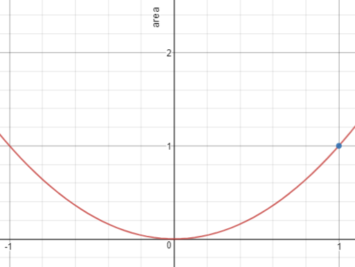
Do the students notice that in the first increase of one in x, there is an increase in of one in y, as well?
Animation 1B explores the function y = 2x2. Look for students to make connections between the pattern of square numbers, the table and graph that pattern produces, and the slightly changed new function. They should notice:
- The areas are twice those of the square numbers.
- The equation is therefore y = 2x2.
- The second order differences are constant at four, twice the second order differences for y = x2.
Graph both functions and look for similarities and differences.
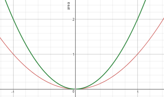
Do the students notice that for y = 2x2 the increase of one from x = 0 results in an increase in area of two, twice that from y = x2.
Similarly, Animation 1C explores the function y = ½x2 using the areas of triangles. Students should notice the areas are half that of the matching square numbers. Ask students to anticipate the likely second order differences and the effect on the graph.
Show all three functions together and ask about similarities:
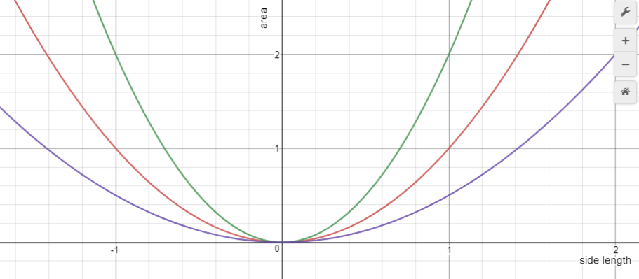
- Do students notice that all the graphs are parabolas with a vertex at (0, 0)?
- Do students notice that changes to the co-efficient of x2 changes the increase in y in the first increment of one in x?
- Can they predict the graphs of other functions in from y = ax2?
- Do they anticipate what will happen if a is negative, e.g. y = -3x2?
Copymaster One gives the students several graphs and requires them to find the function. Insist that they substitute the x and y values for the points they are given to check that their equation works. Students might appreciate access to an online graphing tool to trial equations before committing them to paper.
Session 2: Parabolas everywhere
In this session students investigate where parabolas are found in the natural and human made world. The apply curve fitting techniques to approximate parabolas and generate equations to model the curves.
Show Animation 2A. This provides four examples of parabolic curves. With each example, encourage the students to predict what the equation for the curve might be. Useful questions are:
- Where is the vertex? What does the location of the vertex tell you about the equation? (If the vertex is located at (0,0) that makes finding the equation less complex)
- How can you adjust the equation y = x2 to allow for the steepness of the curve? (Vary the co-efficient of x2)
- How could we check to see how accurate our equation is? (Substituting the x and y values of any points on the curve that are given)
A sensible location for the vertex is (0, 0) since the equation will be in form y = ax2. Only the scale factor a must be found. That factor can be estimated by looking at the increase and decrease in y for the one unit increase in x from zero to one. The equation can be adjusted to allow for a shift in the vertex to (p, q) using the formula y = (x – p)2 + q. This vertex form will be explored later through curve fitting in Session Three.
Copymaster Two gives eight scenarios of a basketball shooter. Thanks to Dan Meyer for this task. Many points on the path of the ball are given, as would appear in time-lapse photography. The challenge is to use the grid system to create a co-ordinate plane and find an equation for the path of the ball. Once the equation is found it allows for prediction about whether the shot will go through the hoop or not. Let your students work in pairs to solve the problems. Look for students to:
- Sketch a reasonable approximation of a parabolic curve.
- Choose a suitable location on the path of the ball for (0,0), preferably the vertex.
- Notice the change in height of the path for an increment of one in the x value either side of the vertex.
- Use the change in height to approximate a in the equation y = ax2.
If time permits, view Animation 2B together. The video shows how Geogebra can be used as a curve fitting tool. You will also need to replay this animation slowly at the start of Session Three so students can follow the steps to create their own curve fitting equation with sliders.
Session Three: Parabolic?
In this session students explore the curve fitting activity more. The main purpose of the session is two-fold:
- Can student learn to distinguish parabolas from non-parabolas?
- Can students understand the effects of manipulating the variables a, p, and q in the vertex form of the equation for a parabola, y = a(x - p)2 + q?
Revisit Animation 2B, working through it until the students create their own slider driven equation and graph. Bring the class together.
Fix p and q on one using the slider.
- What happens to the graph as a is varied? (a acts as a scalar that changes the slope of the parabola. Note that slope is not constant as we saw in Session One).
- How do I invert a parabola? (Change the sign of a)
Fix a and q at one.
- What happens as p changes? (The parabola translates horizontally in the same direction way as the change in value of p)
- Why is it that making p more positive shifts the parabola to the right? (and the opposite direction for negative changes)
This feature of the vertex form is hardest to comprehend, especially given that (x – p) is squared. One way to explain this is to focus on the vertex. For example, in the equation y = (x – 4)2, the x value must be four to create the same effect as x = 0, in the equation y = x2. In the equation y = (x + 4)2, the x value must be negative four to create the same effect as x = 0, in the equation y = x2.
Similarly fix a and p to show that changes in q result it vertical translations of the vertex.
Provide your students with access to these 6 image files. Download zip file (332KB).


Ask your students to insert each image into the parabola graphing tool they have created. Their challenge is to see if they can find a quadratic equation that models each curve. It may be that some curves are not parabolas so a good fit may be difficult.
The path of a projectile under gravity is close to parabolic so the dolphin jump, and fountain jets are good examples. Dams, and other human-made structures, are often parabolic so stress is shared evenly along the curve. Paths of planets, moons and comets are ellipses though they appear close to parabolic in parts.
Session Four: Braking Distances
In this session students explore the quadratic models that lay behind simulators of braking distance. The breaking distance of a car has a quadratic, not linear, relationship with speed. Understanding the effect of speed is critical to road safety awareness of your students. All through the lesson notes, speed is used to indicate the relation between distance and time, but velocity may also be used instead.
- How long does it take a car to stop?
This is an ambiguous question since length could relate to time or distance. Students should suggest that braking distance depends on many factors such as speed and mass of the car, condition of the road (wet/dry, rough/smooth), attention of the driver, the grip of the tyres and quality of the braking system. Make a list of factors.
- We are going to focus on speed to start with. How do you think speed will affect braking distance?
- Will the relationship between speed and braking distance be linear or non-linear? Why?
Invite students’ ideas about the model. Braking distance is made up of reaction distance (linear relation with speed) and braking distance (quadratic relation with speed).
There are many braking simulators and braking distance calculators online. You may like to find one of these and collect your own data or you may prefer to use the data in the table below.
Student should notice that the reaction distance is twice as much for 32 km/h as it is for 64 km/h, but braking distance does not increase in a linear way. This finding is obvious by looking at the differences in braking distance between 32, 48 and 64 km/h.
| Speed (kilometres per hour) | 32 | 48 | 64 | 80 |
| Reaction distance | 6 | 9 | 12 | 13 |
| Braking distance | 6 | 14 | 24 | 31 |
Ask the students to work in pairs to find the relation between speed in km/h and braking distance in metres. Provide the hints that the relation is quadratic and that the braking distance for 10 km/h equals 0.6 m. Students may use difference methods or curve fitting using an online tool or graphics calculator. Since braking distance at a speed of 0 km/h equals 0 m the vertex is at (0,0) which makes curve fitting quite easy.
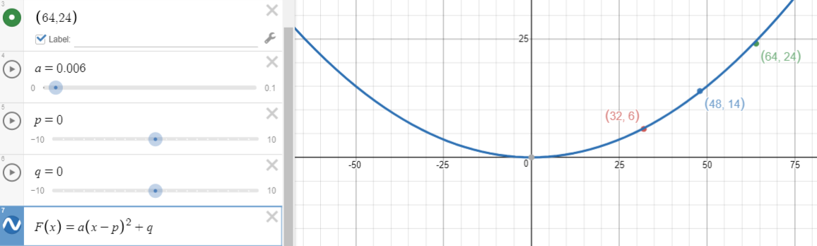
Alternatively, students might use speed in kilometres per hour and apply a difference method. Imagine the speed is divided by ten (or multiplied by 0.1). The increase for y = x2 between x = 0 and x = 1 is 1, so the hint indicates the scalar is 0.6 once s is divided by ten. The equation is Bd = 0.6(s/10)2 = 0.006s2.
- What is the formula for total stopping distance?
Reaction distance and braking distance need to be combined. Let the students work on finding a formula. Since the formula for reaction time is linear students need to look for constant difference.
- As speed increases by 16 km/h what happens to reaction distance? (increases by 3 metres)
Therefore, in the standard formula, y = mx + c, what is m? (3/16).
- How can we find c? (substitute into the formula the values for s and Rd from any point on the curve. For example, using (32, 6) gives 6 = 3/16 x 32 + c, so c = 0. As the curve goes through the origin this must be true).
The formula for total braking distance is the sum of reaction and braking distances;
Td = 3/16 s + 6/1000 s2.
The formula is based on an assumption about the co-efficient of friction between the car wheels and the surface. Some sites give the braking distance for 10 km/h as 0.4 m meaning they use a higher co-efficient of friction.
Let your students investigate what happens to reaction, braking and total stopping distances as conditions are changed.
In wet conditions the co-efficient of friction is less so the braking distance at 10 km/h is 8 metres. Accordingly, the braking distance equation becomes Bd = 0.008s2 and the reaction distance stays the same. Both mobile phone and drunkenness effect the reaction distance. Mobile delays reaction time so the equation for reaction distance becomes Rd = 13/32 s or 0.41s. Drunk driving decreases reaction time so reaction distance is modelled by Rd = 10/32 s or 0.31s. In both cases the braking distance stays the same.
The graph below illustrates stopping distances at different speeds.
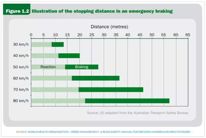
Create a data table of reaction distance and braking distance for different speeds shown on the graph. There will be minor variations in reading from the graph due to rounding.
| Speed (km/h) | 30 | 40 | 50 | 60 | 70 | 80 |
| Reaction distance (m) | 8 | 11 | 14 | 17 | 19.5 | 22 |
| Braking distance | 5 | 8 | 13.5 | 35 | 52 | 66 |
Ask:
- How does this data connect to the previous data?
- What are the implications for safe driving?
Session Five
In this session students apply their knowledge of quadratic functions to maximise profit for a business. Functions are commonly used in economics to model profit and loss scenarios. The attached PowerPoint drives the lesson structure.
Slide One asks students to create a demand function for Gina’s lemonade.
- Is the demand function linear? How do you know? (Yes. There is a constant rate of change – 100 less people for every 50-cent increase in price per glass)
- Which variable goes on the horizontal (x) axis and which variable goes on the vertical axis (y)? (There is a convention in economics that price in dollars goes on the vertical axis and quantity goes on the horizontal axis.)
- What will be the y-intercept and slope of the graph? How do you know? (At $5.00 per glass no lemonade will be sold. So (0, 5) is the y-intercept. As the price decreases by 0.5 and extra 100 glasses are demanded so the slope is 0.5/100 = 0.005 or 5/1000.)
Using a graphing tool or graphics calculator students should be able to graph the function and record it as an equation, using p and q for price and quantity respectively. Slide Two shows the graph.
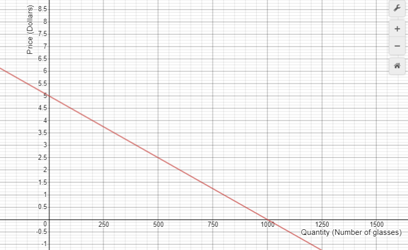
The function can be written as p = 5 – 0.005q or p = -0.005q + 5. For the purposes of modelling revenue, it is also important that quantity is considered as a function of price.
How might we express quantity as a function of price? (make q the subject of the equation)
Students might apply their algebra skills to make q the subject, that is, express q as a function of p. Be aware that students may find division by -0.005 or -5/1000 challenging.
p = 5 – 0.005q
→ p – 5 = -0.005q
→ (p – 5)/-0.005 = q
→ 1000(5 – p)/5 = q
→ 200(5 – p) = q or → 1000 – 200p = q
It is likely to be easier to consider the information contained on Slide One again. The quantity demanded starts at 1000 glasses when p = 0 and decreases by 200 glasses for each dollar increase in price. That observation leads more naturally to 1000 – 200p = q.
Slide Three of the PowerPoint discusses how Gina might model her total revenue.
- How could Gina work out how much money she will take in total? (That will be the product of quantity and price, number of glasses sold x price in dollars).
- How might her revenue equation be written? (t = p x q)
- Can the equation p = 5 – 0.005q be combined with t = p x q in some way? (Substituting the first equation into the second gives t = q (5 – 0.005q).
- What kind of function of price will total revenue be? What will the graph look like? (It will be quadratic since q (5 – 0.005q) = 5q – 0.005q2. The graph will be a negative parabola.)
Students might graph the equation and find out the quantity that maximises Gina’s revenue.
Of course, Gina is more interested in the price to charge that maximises her revenue.
Can the equation p = 5 – 0.005q be combined with t = p x q in some way? (Substituting the first equation into the second gives t = p (1000 – 200p).
- What kind of function of price will total revenue be? What will the graph look like? (It will be quadratic since p(1000 – 200p) = 1000p – 200p2. The graph will be a negative parabola.)
Slide Five shows the graph of total revenue as a function of price.
- For what prices does Gina take in no money? (0 and 5 dollars)
- Why is that true? (She gives the glass away for free or nobody buys any)
- At what price is her total revenue at its highest (maximised)? ($2.50)
- Is that the price she should charge or are there other things to consider? (Gina has not thought about her costs)
Slide Six shows Gina’s costs.
Some of her costs are fixed and some are variable because they depend on the number of glasses she sells. Divide the costs into fixed (site and refrigerator hire, electricity, and loan repayment) and variable (lemons, ice, glasses, sugar). Total these two categories of cost.
- Can you write a function for cost as a function of quantity, q? (c = 280 + 1.2q, since Gina has $280 in fixed costs and $1.20 variable cost per glass)
- Let’s show both revenue and cost functions on the same graph. How will we find out the quantity that maximises her profit?
Let students graph the Total Revenue and Total Cost functions on the same graph. The quantity at which the difference between revenue and cost is greatest gives the maximum value. It is quite hard to establish that quantity from the graph.
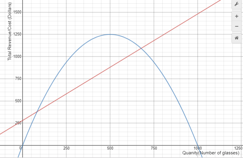
Animation 5 shows how the functions can be combined to find the quantity at which Gina maximises her profit (380 cups). Gina does not control quantity, she manipulates it by fixing her price.
- What price should Gina charge so she sells 380 cups of lemonade? (380 is substituted as the value for q into p = 5 – 0.005q. This gives a price of $3.10 per cup.)
Copymaster Three gives students a chance to apply what they have leaned to a different business scenario. Can your students create revenue and cost equations to maximise profit?
Hello families and whānau,
This week our class is learning about algebra. We will be using an area model to help us to expand and factorise quadratic expressions. Those skills are very important if we want to succeed in future mathematics, particularly calculus.
Please take the opportunity to discuss with your student what they are learning. They may be willing to demonstrate how they solve some of the problems from class.