Probability Distributions
This unit introduces students to concepts that are important in probability, including the probability function. All the ideas are important as a base for future learning in this area of mathematics.
- Explain what a probability distribution is.
- Explain how probabilities are distributed.
- Calculate what happens to the distribution when variables are summed.
- Calculate expected number from theoretical probabilities.
- Appreciate the difference between theoretical and experimental probabilities.
The probability distribution of a discrete random variable is a list of probabilities associated with each of its possible values. It is also sometimes called the probability function or the probability mass function. So, for example, if we were to toss two coins, we know that there is an even chance of getting heads or tails for each. Therefore the probability distribution of the event "tossing two fair coins" looks like this: Two tails, One head and one tail, Two heads 1/4 1/2 1/4. There is a one in four chance that both coins will be tails, a one in 2 chance that one coin will be tails and the other tails, and a one in four chance that both coins will be tails.
The emphasis in this unit should be on working slowly, taking the time to let the students grasp the ideas that underlie the activities presented.
- Coins
- Dice
- Spinners
Session 1
This session aims to give the students a feel for what a probability distribution is, and to introduce them to 2 methods of simulating variables.
-
Group the class in 3s.
-
Issue each group with a pair of dice and pose a contextual question that will form the scaffolding for the skills and ideas they will cover in this session. If four friends are playing a two dice board game that requires each player to roll a double (difference of zero) before they can start, what is the expected number of rolls for all four of the players before everyone has started?
-
They investigate the difference between the two numbers when the pair is rolled (difference is simply larger minus smaller).
What does investigation mean in this situation?
What all the possible answers?
Are some more likely than others? How do you know?
Which are most likely?
Which are least likely?
What is the probability of each outcome (that is, what is the probability that the difference will be 0, 1, 2, 3, 4, 5)?
Leave students to their own methods. -
Discuss the results as a class:
What answers did you find?
How did you go about it? -
If no one suggested a 6x6 table show them how one can be constructed.
1 2 3 4 5 6 1 0 1 2 3 4 5 2 1 0 1 2 3 4 3 2 1 0 1 2 3 4 3 2 1 0 1 2 5 4 3 2 1 0 1 6 5 4 3 2 1 0 -
From the table the probability distribution can be found.
| 0 | 1 | 2 | 3 | 4 | 5 |
| 1/6 | 5/18 | 2/9 | 1/6 | 1/9 | 1/18 |
-
Discuss the context question (2) with the class, noting the difference between probability and expected number.
-
Set up a simulation to model the context question (2). For this, random numbers from 1-18 can be used (on a calculator, 18RAN# +1) and each student in the class should run the simulation until every player is on the board. (Note that once a player is on the board, they will continue to roll the dice when it is their turn).
-
Regroup and review the simulation. Find the mean of the students' results for the number of rolls it took before all players were on the board (including players on the board taking their turn). Use this result to compare theoretical and experminental probabilities and to compare probabilities with expected number.
Session 2
This session aims to investigate the sum of 2 variables.
-
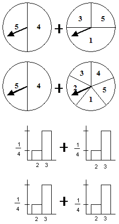
Put the class in groups to investigate the sum of these two variables. Ask them to show the distribution of the sum as a table and as a graph.
-
Class discussion to see the methods and solutions found. Solution to show class: Divide each spinner into 12ths (why 12ths?). Hence complete 12x12 table.
| 1 | 1 | 1 | 1 | 2 | 2 | 2 | 2 | 3 | 3 | 3 | 3 | |
| 1 | 2 | 2 | 2 | 2 | 3 | 3 | 3 | 3 | 4 | 4 | 4 | 4 |
| 1 | 2 | 2 | 2 | 2 | 3 | 3 | 3 | 3 | 4 | 4 | 4 | 4 |
| 1 | 2 | 2 | 2 | 2 | 3 | 3 | 3 | 3 | 4 | 4 | 4 | 4 |
| 2 | 3 | 3 | 3 | 3 | 4 | 4 | 4 | 4 | 5 | 5 | 5 | 5 |
| 2 | 3 | 3 | 3 | 3 | 4 | 4 | 4 | 4 | 5 | 5 | 5 | 5 |
| 2 | 3 | 3 | 3 | 3 | 4 | 4 | 4 | 4 | 5 | 5 | 5 | 5 |
| 3 | 4 | 4 | 4 | 4 | 5 | 5 | 5 | 5 | 6 | 6 | 6 | 6 |
| 3 | 4 | 4 | 4 | 4 | 5 | 5 | 5 | 5 | 6 | 6 | 6 | 6 |
| 3 | 4 | 4 | 4 | 4 | 5 | 5 | 5 | 5 | 6 | 6 | 6 | 6 |
| 3 | 4 | 4 | 4 | 4 | 5 | 5 | 5 | 5 | 6 | 6 | 6 | 6 |
| 3 | 4 | 4 | 4 | 4 | 5 | 5 | 5 | 5 | 6 | 6 | 6 | 6 |
| 3 | 4 | 4 | 4 | 4 | 5 | 5 | 5 | 5 | 6 | 6 | 6 | 6 |
-
Ask the students to use the table to find the probability distribution.
-
Pose the following problem to groups.
Make a spinner that simulates, in one spin, the sum of these two variables.
Session 3
Continue the investigation of the sum of 2 variables.
-
Group the class. For each of the following pairs of variables (1) find the distribution of the sum (2) show the distribution as both a table and a graph (3) construct a spinner that simulates the sum in a single spin.
-
If time remains challenge students to make up their own examples.
-
Class discussion. How would you go about adding 3 variables?
Session 4
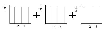
This session has two aims: (1) to investigate the distributions when uniform variables are added, and (2) add three variables. Another way to show uniform variables is on a bar graph as the illustration below shows.
-
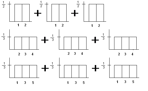
In groups add the following pairs of uniform variables. Graph the distribution of the sum in each case.
-
Class discussion. How would you add the three variables in.
Solution: tree diagram.

Therefore the probability distribution is:

-
Pose the following examples for students to work on:
-
Pose the following question for a class discussion: How would you add the 3 variables in the example below?
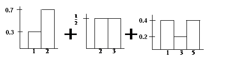
Share strategies and approaches:
-
Ask the students to, in pairs, complete the previous example and draw the distribution of the sums.
Session 5
This session uses the above ideas to answer word problems.
-
Pose the following problems for the class to solve in small groups. Ask the students for their ideas on how to proceed.
Problem 1: Three seeds are planted. Each has probability 0.3 of growing. Draw the distribution of the number of seeds that grow.
Problem 2: Three lightbulbs are switched on for a month. The chance of any one of the bulbs blowing during this period is 0.2. Find the probability that all will blow during the period; two will blow; one will blow; none will blow. Graph the distribution.
Problem 3: It is known that 10% of torches made by a particular factory are defective. If you buy three torches, what is the probability distribution for the number of them that will be faulty? -
Share methods and solutions.
-
Make up your own problem along the same lines.